ESMD Course Material : Fundamentals of Lunar and
Systems Engineering for Senior Project Teams, with Application to a
Lunar Excavator
Contact: David Beale, dbeale@eng.auburn.edu
Contact: David Beale, dbeale@eng.auburn.edu
|
|
Computer-Aided
Engineering Tools
David Beale
Contents
Modeling is often used in the formulation phases of Systems Engineering,
and it is particularly applicable to lunar excavator design because
prototypes cannot be tested on earth under the exact operational
conditions expected on the moon. Lunar
gravity, radiation, wide temperature fluctuations and regolith are
factors that drive excavator design, and it is all but impossible to
test a new product under these lunar conditions. However,
simulations can be performed that impose the lunar conditions, then
hopefully the simulation’s output will be representative of how the
product will perform under lunar conditions. Since each university will have its preferred software suite, this presentation is meant to show potential applications rather than be a tutorial for a specific software. Graphical design of hardware is performed with a Computer-Aided Design (CAD) drawing package capable of graphically representing parts based on part features. Next the designer can assemble the parts to make a component or a system by applying assembly relationships. Next the assembly can be examined for fit and function by testing a “virtual” prototype before producing a physical prototype.
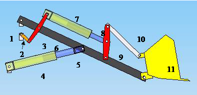
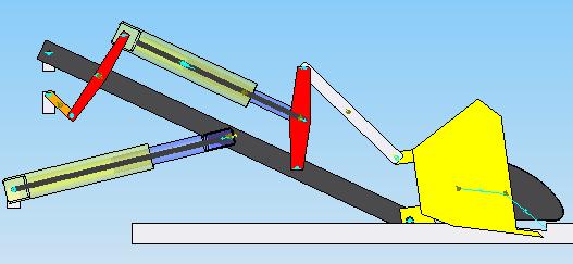
Figure 1‑1. Excavator assembly in Solid Edge To demonstrate the process, a CAD package (Solid Edge V20) was used to draw and assembly an excavator shown in Figure 1-1. Individual parts were created first, and then assembly relationships applied. The excavator would be pinned at three points on the left side of the figure to a rover (for this demonstration they are attached to ground part 1). The figure shows 12 pin (or revolute) joints and 2 translational joints in the cylinders. Each joint removes 2 degrees of freedom. With 10 moving parts, Gruebler’s equation calculates this system to have 2 degrees of freedom. Hence two actuators (e.g. linear motors) will be able to operate this system, and obvious locations for these would be inside the cylinders, between parts 4 and 5, and 7 and 8. · Actuator power and force requirements, and link dimensions sized for the intended lifting and digging operation. The digging force mathematical model (Chapter 5) can be added as an applied force. Use a multibody dynamics simulation software here like ADAMS. · Stresses throughout the mechanism parts induced by digging, from combined multibody dynamic simulation and finite element analysis. · The temperature of any material point on a part (created by solar radiation and the environment), by finite element analysis. · Thermal stresses and strained induced by temperature differences within a part, and across part joints, again using finite element analysis. Input boundary conditions determined by methods presented in “thermal control” chapter 7. · Control laws that define actuator motion based on sensor input, to automate and/or monitor the digging operation. Use a multibody dynamics and/or a control system design software like MATLAB.
Multibody
Dynamic Simulation of the Digging Process
The parts and assembly of Figure 1-1 were built using Solid Edge
V20. Dynamic
Designer is a multibody simulation dynamics software interface that
is an add-on software to Solid Edge. It is offered at no cost to
students through Dynamic Simulation Technologies at http://interactivephysics.design-simulation.com/DDM/SolidEdge/faq.php (however
you will need to make sure your particular CAD package will support
it). The
multibody dynamic simulation engine of Dynamic Designer is ADAMS,
which could be directly accessed by importing your CAD assembly into
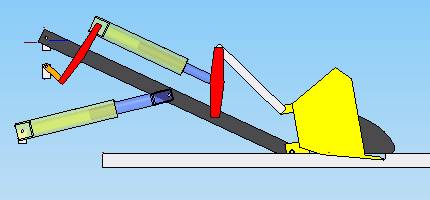
Figure 1‑2. Starting position, side view
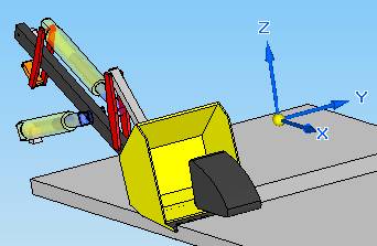
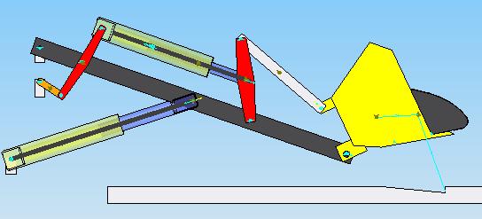
Figure 1‑3. Starting position, isometric view
Figure 1‑4. Prescribed splined displacement vs. time, top cylinder
Figure 1‑5. Prescribed splined displacement vs. time, bottom cylinder
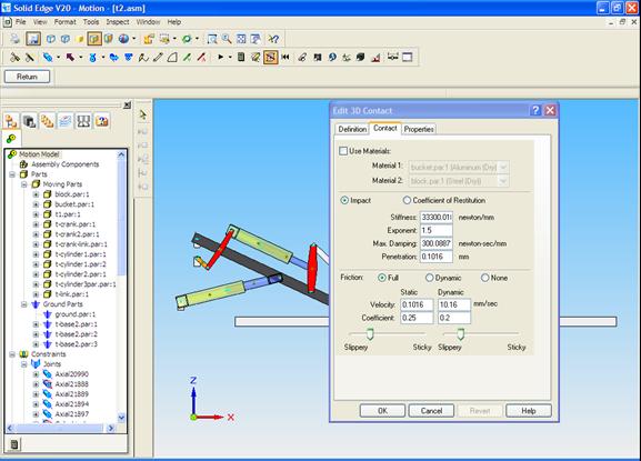
Figure 1‑6. Bottom cylinder length vs. time The simulation starts by lifting a rock already in the shovel. A “contact force” (Figures 1-7 and 1-8) is defined between the rock and the shovel since no joint exists between the rock and the shovel. The important parameter values here are the stiffnesses of the contacting elements, i.e. the steel shovel and the rock. Similarly a contact force is created between the rock and the ground. Sharp spikes in Figure 1-8 are often numerical error, and can be reduced by increasing accuracy of the numerical integration and increasing damping in the contact. The spike near t=0 is due to an impact as the shovel moves upward and contacts the rock. The full sequence of motions is shown in Figure 1-11 through 1-16.
Figure 1‑7. Window for defining contact force parameters between shovel and rock
Figure1‑8. Contact force between rock and shovel
Figure 1‑9. Actuator force in lower cylinder
Figure 1‑10. Long beam to shovel revolute joint reaction force in Z (vertical direction)
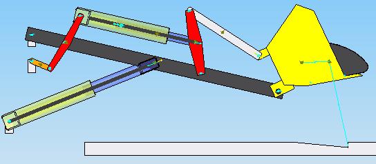
Figure 1‑11. Simulation at t=0
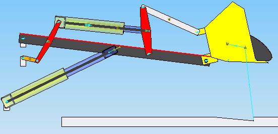
Figure 1‑12. Simulation at t=1 second
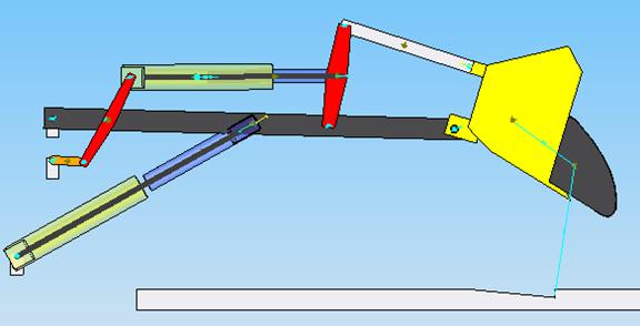
Figure 1‑13. Simulation at t=2 seconds
Figure 1‑14. Simulation at t=3 seconds
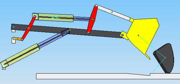
Figure 1‑15. Simulation at t=4.4 seconds
Figure 1‑16. Simulation at t=5 seconds |
||||||||||||||||||||||||||||||||||||||||||||||||||||||||||||||||||||||||||||||||||||||||||||||||||||||||||||