Thermal Considerations of Lunar Based Systems

Daniel K. Harris

1.       Scope

The scope and breadth of this chapter will cover the least rudimentary components of thermal design and analysis as applied to lunar based systems.  This chapter is as self-reliant and all inclusive as could be reasonably expected while minimizing the volume of this chapter.  It is intended to give only the briefest of outlines of the thermal science behind the engineering described.  The interested reader is guided to references that will give more detail in the physics behind the heat[1] transfer modes and mechanisms used here.  The reader of this section is assumed to have a baccalaureate in engineering or physics and is not familiar at all with heat transfer and thermal design.  The reader is assumed to be interested in only the most general enveloping analysis to guide his or her design of a mechanical structure located and based on the lunar surface for extended time periods.  The design methodology is presented in an easy to mimic style.  The unique lunar environment and the challenges it presents are offered in a simple to understand approach.  The chapter concludes with a case study giving the reader some final guidance, and hopefully confidence in designing a thermal management approach for whatever they are intending to deploy on the surface of our moon.    Radiation

2.       Purpose

The objective of this chapter is to introduce the skill of calculating temperatures and heat flux values for given boundary conditions on the lunar surface.  This skill will primarily consist of adequately modeling radiation surface interchange phenomena in both the UV and IR portions of the radiation spectrum.  The methods taught here will involve “hand” calculations using spreadsheets or other easily available computer tools.  More sophisticated techniques requiring commercially available software are referenced but not described in detail.  Since the lunar diurnal cycle has a period of approximately 28 Earth days, steady state calculations are the most appropriate and are therefore stressed throughout this chapter.  The engineering design methodology applied here is to identify worst case hot and cold conditions.  Once these two worst case extremes have been identified the engineer has to see how his or her system can operate and survive under these two conditions.  Thermal remediation techniques and options will also be taught in this chapter.  It will then be up to the engineer to “engineer” the system within the defined lunar conditions. 

 

1.       Introduction

You may not be aware of just how large a role our atmosphere plays in everyday life as a medium to transport heat and mass.  Not only does the atmosphere around us transport almost all of the thermal energy to and from all entities, but it also plays a vital role in moderating temperatures and diffusing (smearing out) large discrepancies in our thermal environment.  Air cooks our food, runs our cars, heats and cools are homes, cools our computers, helps our bodies regulate its temperature, and on and on.  Needless to say without an atmosphere thermal environments become very difficult for anybody or anything to function within.  Thermal design and management is challenging enough in an atmosphere.  But, in the absence of an atmosphere (vacuum) it becomes more critical and a main component of any design.  Further, because of our everyday experiences are from a perspective of being immersed in an atmosphere, most aspects of a space thermal environment are difficult to predict and in many cases non-intuitive.  Therefore, we cannot rely on our good judgment or everyday experiences when designing a system for operation in space, or worse yet, on the surface of the Moon. 

a.             Heat conduction is the mechanism for heat transfer through bulk solids and fluids.  It is a gradient transport type of phenomena and is described by Fourier’s empirical Law, which in its differential form is as shown here. 

Once taken to its integral form it takes on the more familiar appearance as,

where k is the bulk material thermal conductivity.  This heat transfer mechanism will not be significant in most situations where an external surface is interacting with the lunar environment.  However, once the system boundary conditions are defined by the interactions with the external lunar thermal environment, conduction heat transfer will be a very significant heat transfer mechanism. 

 

b.            Radiation heat transfer phenomenon is the dominant heat transfer mode on the lunar surface.  Unlike conduction heat transfer, which occurs inside a bulk solid or fluid, radiation heat transfer is a surface phenomenon.  Radiation heat transfer occurs over the long wave length, infra-red, part of the electromagnetic wave spectrum.  All matter rejects and receives thermal energy via thermal radiation.  The radiating power of any matter at a non-zero temperature is given by the Stefan-Boltzmann equation,

where A is the surface area, e is the emissivity, T is the absolute temperature, and s is the Stefan-Boltzmann constant (5.670 51 x 10^-8 W/m K⁴).  The thermo-optical property of the surface called emissivity determines the ability of the surface to both transmit and absorb (under the gray body assumption) thermal radiation and lies between zero and unity.  A perfect thermal radiating surface will have an emissivity of one and is termed a ‘blackbody’.  While the physics behind this phenomenon is quite complex, simple averaged values are used for the emissivity.  Surface emissivity can be both wave-length (spectrally) and directionally dependent.  Therefore, for the purposes of engineering calculations values for the surface emissivity are used that have been averaged (integrated) over all possible wavelengths over all directions of a hemisphere.  Bodies with an emissivity that is spectrally independent are called ‘gray bodies’, where the infra-red emissivity is assumed equal to the infra-red absorbtivity.  This is known as the gray body assumption and is quite adequate for most common surfaces. 

The interchange between two or more surfaces requires an optical analysis to determine the view factor between the two surfaces.  The view factor between two surfaces (say surface i and surface j) is identified by F_ij.  It also has a value between zero and unity.  It represents the percentage of view one surface has to another surface.  It is quite difficult to determine the view factor even between two simple geometries.  Therefore, a catalog of common surface geometries is usually needed and the analyst can simplify the calculations in order to estimate the view factor.  See for example [Modest, 1993], pp. 780-794 for some of the most common shapes encountered.  Once the view factor is determined then the (net) radiation interchange between the surfaces at their respective temperatures (T_iand T_j) is given by the following equation. 

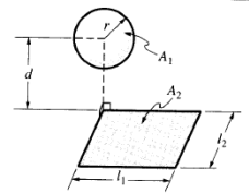
As an example we’ll compute the radiation heat transfer between a sphere of radius r and a plane rectangle of dimensions 2l₁ by 2l₂, separated by a distance d (measured from the sphere’s center to the plane rectangle) and centered directly ‘under’ the sphere. 

Figure 00: Geometry under analysis, where only ¼ of plane is shown due to symmetry.)

As found in [Modest 1993] on page 792, item 47 shows the view factor for this geometry under consideration as follows:

In this example we’ll let the dimensions of the rectangle plane be 2d by 2d.  Therefore, both l₁ and l₂ are equal to d, giving D₁ and D₂ both equal to unity.  This gives F_1-2 a value of,

This gives the view factor of the sphere to one-quarter of the rectangle; refer to Figure 00.  The view factor of the sphere to the entire plane rectangle is 4 times as much, or 0.1024.  This can be interpreted as saying that 10.24% of all the radiant energy leaving the sphere will be incident onto the plane rectangle.  Now there exists a handy relationship for view factors between two surfaces that allows the direct determination of the view factor from the plane rectangle to the sphere (which is necessarily not the same value).  This is known as the reciprocity relation.

This means that the view factor from the plane rectangle to the sphere is found as

Now, if we let d=2r, then F_2-1 becomes equal to 0.0804.  Only roughly 8% of the energy leaving the plane rectangle is incident upon the sphere. 

As an extension to more than two surfaces an additional relationship is useful.  The sum of all view factors for each surface comprising a multi-surface enclosure is unity.  This means that for all surfaces comprising the enclosure, the following relationship holds for all N surfaces.

This is known as the summation rule.  In fact, for an enclosure comprised of N surfaces a total of N² view factors is needed.  However, only N(N-1)/2 view factors need to be determined directly by invoking the reciprocity relation and the summation rule. 

Carrying this example calculation forward, let’s consider values for the temperatures and emissivities.  This will allow for the last component of a radiative heat transfer calculation to be explained.  The heat transferred between these two surfaces will be found using the concept of radiosity.  Radiosity is essentially the concept whereby a surface can have thermal energy that it radiated reflected back onto its surface.  It is a concept needed for thermal radiation calculations of multiple surfaces.  Without going into too much detail only the basics of radiosity network analyses (also known as Oppenheim networks) is described here. 

For gray and diffuse (directionally independent) surfaces the emissivity e is assumed to be equal to the infra-red absorbtivity a  (not to be confused with the a representing the UV absorbtivity), and therefore the reflectivity r of the surface is equal to (1-a) or (1-e).  The radiosity of a surface J_i can be expressed as the following where G_i is the incident radiation onto the surface and E_bi is the blackbody radiating power of the surface at its temperature, given as e_isT_i⁴.

Therefore, the net radiative heat transfer rate from a surface is given as follows. 

Hence, if the emissive power that a surface would have if it were black exceeds its radiosity, there is net radiation heat transfer from the surface; if the inverse is true the net transfer is to the surface. For a network of surfaces that can view one another the radiation balance for each surface can be represented as follows.

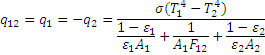
Using this relationship for each surface a network can be generated for all the surfaces and a non-linear system of equations is produced that can be numerically solved.  For a simple two surface interchange the net radiation between the two surfaces is found to be as follows. 

Since the objective of this chapter is to describe analyzing a lunar thermal environment, we have to leave the radiation heat transfer discussion and return to the application of these principles described.  Most design calculations that try to define both the worst case hot and cold environment analyses will usually involve only simple surface geometries interacting with other nearby surfaces including the lunar surface, and space.

c.                   Ultraviolet absorption as a result of direct or reflected sunlight incident on external surfaces solar absorption is another lunar surface phenomenon that needs attention.  Just as was the case for infra-red radiation heat transfer discussed in the previous section only the rudiments are covered here for design purposes.  Any surface when exposed to ultraviolet (uv) radiation will either reflect (r), absorb (a)or transmit (t)the energy: note that r+a+t=1.  For most cases on the lunar surface (except for windows) the transmitted uv energy will be zero.  The energy will be either reflected or absorbed and converted to heat.  The amount of heat generated on a surface due to absorbed uv energy (i.e. sunlight) is simply the incident radiation flux onto that surface times the uv absorption coefficient a, 

where A is the surface area, a is the absorbtivity, and G_solar is the incident solar flux (ca. 1353 W/m² on the lunar surface).  Recall that the emissivity covers the infra-red region of the electromagnetic spectrum while the absorbtivity discussed here is for the ultra violet region.  This is not to be confused with the gray body assumption discussed previously where a surface’s emissivity can be assumed equal to its absorbtivity over the infra-red region.  It is imperative that these two absorbtivities not be used interchangeably.  An example will help demonstrate the point.

As an example let’s compute the resulting temperature of a clear anodized aluminum surface exposed to direct sunlight on the lunar surface and viewing only deep space, (i.e. no view to the lunar surface).  A simple heat balance applied to the surface gives that the absorbed uv energy must equate to the infra-red energy radiated away from the surface. 

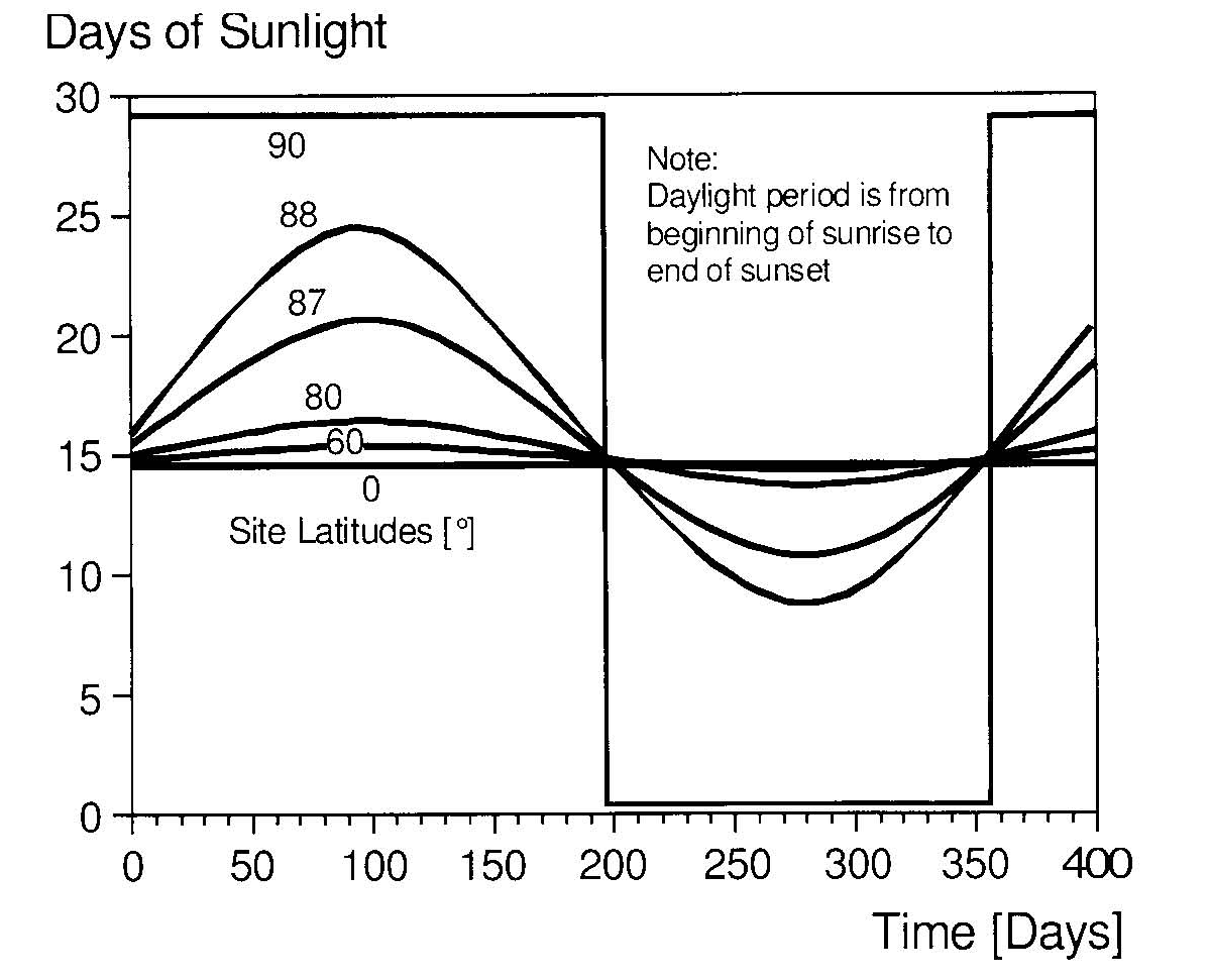
Using values of a=0.35, e=0.76 and G_solar=1353 W/m² gives a temperature of 323.8 K.  As an interesting aside the equilibrium surface temperature exposed to direct sunlight with an a/e of unity is 393 K, and with an a/e = 0.25 is 277.9 K.  This technique of computing equilibrium temperatures will be expounded upon further when discussing thermal analysis of lunar based devices. 

Solar Entrapment - Finally, a word of caution about solar entrapment should be included here.  Solar entrapment occurs when direct solar energy is incident upon an open enclosure or cavity.  What happens is that the solar energy is almost all trapped due to multiple reflections inside the cavity while the view factor of the inner surface (which is heating up from the absorbed solar energy) to the outside environment (the sink) is very low.  In other words, the inner surface of the cavity sees mostly itself and therefore has very low emissive power to the outside environment.  The result of this entrapped solar energy without any way of being effectively radiated away is for the surface to become extremely hot.  Therefore, it is always advisable to avoid designing any cavity like structure that can be exposed to direct (or even reflected) sunlight.

2.       Lunar Thermal Environment

Quite a lot has already been discussed regarding the lunar environment in an earlier chapter.  This section will collect the pertinent information needed to perform a complete analysis.  While redundant, it is intended to pull together in all one place the tables and properties needed for lunar specific thermal analyses.  Essentially, there are three areas of interests in defining the lunar thermal environment: the length of lunar nights, the direct and reflected solar flux, lunar soil temperatures, and associated lunar surface IR energy.

a.                   Lunar day cycles are quite long when compared to our own.  In fact, at the equator the lunar day lasts 14.75 Earth days out of the 29.5 Earth days in the lunar day.  Also, this daylight length period is a weak function of latitude due to the very slight angle (1.533^o) of the Moon’s polar axis (spin axis) off the solar ecliptic. Comparing that with the Earth’s orbit inclination of 23.5° we can understand why the Moon has no annual seasons.    Therefore, only at or very near the Moon’s poles (within 5 to 7 degrees of the pole) are there significantly long daylight and dark periods.  At the poles the daylight periods will last 180 Earth days.  The Figure below shows the length of daylight periods as a function of latitude for the northern hemisphere as taken from [Eckart 2006].

Figure 01: Lunar Diurnal Cycle as taken from [Eckart, 2006], pg. 118.

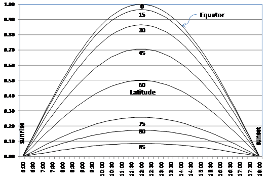
b.                  Solar light on the lunar surface is quite different in nature than that which we are used to on the Earth.  This is due to the lack of any lunar atmosphere which scatters sunlight before reaching the surface.  Therefore, the solar energy incident on any lunar surface is highly directional and therefore depends more strongly on latitude and lunar hour.  For a zenith facing surface the percentage of full solar flux incident (solar flux fraction) is the product of the sine of the local lunar time angle and the cosine of the latitude, where the equator is 0 degrees latitude.  The local lunar time angle is defined as 0 degrees at sunrise, 90 degrees at noon (sub-solar), and 180 degrees at sunset.  The resulting solar flux fraction for a zenith surface is shown here in Figure 02.  Additionally, for an east oriented surface (leading face) the percentage of full solar flux incident (solar flux fraction) is the product of the cosine of the local lunar time angle and the cosine of the latitude, where (again) the equator is 0 degrees latitude is the equator.  The solar flux fraction is a maximum value at sunrise and vanishes at local noon for the remainder of the orbit.  The solar flux fraction is shown below in Figure 03. Consequentially, for a west oriented face (trailing face) the solar flux fraction is the opposite where the flux starts at noon and peaks at sunset.  This is shown for both faces in Figure 03. 

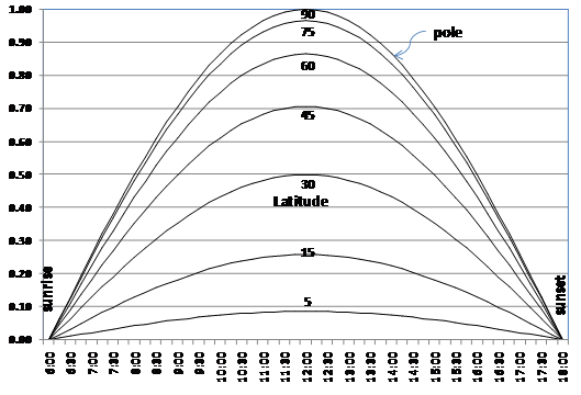
Figure 02: Incident Solar Fraction on a Zenith Oriented Surface dependence upon both Latitude and Local Lunar Time.  The Lunar Local Time is defined as sunrise at 6:00 and sunset at 18:00, which represents 14.75 Earth days.

Finally, for a north oriented face in the southern hemisphere, or equivalently, a south oriented face in the northern hemisphere, the percentage of full solar flux incident on the surface is similar in form to Figure 02 for the zenith face only the latitude dependence is reversed.  The resulting solar flux fraction graph is shown in Figure 04. 

 

Figure 04: Incident Solar Fraction on a North Oriented Surface in the southern hemisphere dependence upon both Latitude and Local Lunar Time.  Note: this graph is identical to that for a South Oriented Surface in the northern hemisphere.  The Lunar Local Time is defined as sunrise at 6:00 and sunset at 18:00, which represents 14.75 Earth days.

c.                   Albedo (the reflected solar energy from the surface) on the lunar surface is only around 7% of the solar flux incident onto the lunar surface.  That is, the lunar surface absorbs almost 93% of all incident solar energy it receives.  This compares to the Earth’s orbital average albedo of 37%.  Therefore, all surfaces exposed to lunar surfaces during daylight periods will be exposed to the lunar albedo, which be assumed as diffuse (directionally independent).  Recall that the absorbed albedo (heat) will be the product of any incident albedo and the absorbtivity.  The incident albedo will also be a function of both the latitude and the local lunar time.  For analysis purposes the solar flux fraction for a zenith oriented face shown in Figure 02 above can be used to find the local albedo by multiplying the fraction found in the figure by 94.7 W/m² (i.e. 7% of 1353 W/m²).  The view factor from the surface to the lunar surface will also be needed in addition to the solar absorbtivity.  Therefore, the total heat generated on a surface by both direct solar and albedo absorption will be as follows.

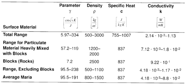
In the equation above the F_solar factor is found in Figure 00 and the geometrical view factor, F_view, will have to be determined based upon the orientation of the surface normal to the lunar surface.

d.                  

Table 01: Lunar Soil Monthly Averages and Ranges, taken from [Eckart, 2006], pg. 143. Temperature Shadowed Polar Craters Other Polar Areas Front Equatorial Back Equatorial Limb Equatorial Typical Mid-Latitudes Average 40 K 220 K 254 K 256 K 255 K 220 – 255 K Monthly Range none 10 K 140 K 140 K 140 K 110 K

The lunar soil temperature is also needed for lunar thermal environment analyses.  The surface soil (regolith and rocks, etc.) on the Moon has a very high diurnal temperature swing between lunar noon and lunar night.  In fact, the temperature on the back equatorial has a range of 140 K to 256 K.  Table 01 below taken from [Eckart 2006] and shows estimated lunar surface temperatures

A first-order estimate of off equatorial variation of soil temperatures as a function of the latitude angle (b) is also given by [Eckart 2006], pg. 143, as follows.

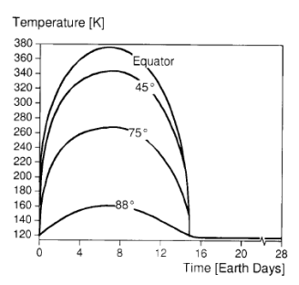
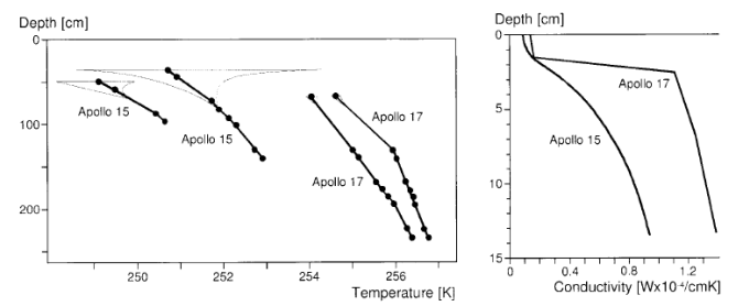
As an alternative, the lunar surface profile temperatures as a function of latitude and local lunar time is shown in Figure 05, as taken from [Eckart 2006], pg. 30]. 

At the Apollo sites the mean temperature 35 cm below the surface are 40 to 45 K above those at the surface.  Figure 06 below shows the temperature and soil thermal conductivity as a function of depth at the Apollo 15 and Apollo 17 landing sites [Eckart, 2006].  Table 02, following gives some important soil thermal parameters and their respective ranges.  In Table 02, g is the thermal inertia of the soil. 

These influences include heat conduction to and from any surface structure, and the infra-red radiation heat transfer interactions with any structures that have an optical view of the surface.  Whereby, the latter is usually the most dominant mode of heat transfer to and from a structure on the lunar surface.  Knowing the lunar thermal environment gives the designer the information necessary to find the environmental thermal loads his or her lunar device will be exposed to on the lunar surface. 

Figure 05: Lunar Surface Temperature Profile at Different Latitudes, taken from [Eckart, 2006], pg. 301.

 

Figure 06: Lunar Soil Temperature and Thermal Conductivity as a Function of Depth at the Apollo 15 and Apollo 17 Landing Sites, as taken from [Eckart, 2006], pg. 140.

Table 02 Lunar Soil Temperature and Thermal Conductivity as a Function of Depth at the Apollo 15 and Apollo 17 Landing Sites, as taken from [Eckart, 2006], pg. 141.

 

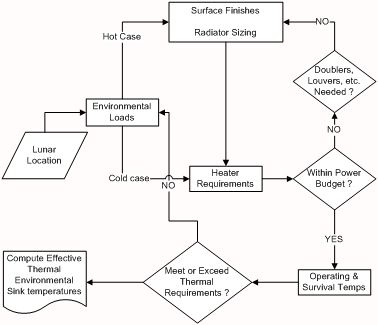
3.                   Thermal Analysis & Approach - The first step needed to design a system capable of operating and surviving on the lunar surface is to define the effective environmental temperatures expected from the defined environmental loads.  The design can then mature to define the exterior surface finishes needed, heat rejection radiator sizing, heater power requirements, etc.  Before an analysis that can direct a thermal design can commence the lunar location, thermal requirements (both operating and survival), and the system power requirements and budget need to be known.  These are the constraints that the mechanical design of any lunar device will have to operate and survive under.  The thermal design approach is shown graphically in the following flow diagram. 

Thermal Design Flow Sequence.

a.                   The thermal requirements (supplied or derived) that are needed in developing a thermal design include the following list:

·         

Table 03: Some Typical Components and Operational Temperature Ranges, as adapted from [Wertz & Larson, 1999], pg. 428. Component Typical Temperature Ranges (°C) Operational Survival Batteries 0 to 15 -10 to 25 Power Box Baseplates -10 to 50 -20 to 60 C&DH Box Baseplates -20 to 60 -40 to 75 Antenna Gimbals -40 to 80 -50 to 90 Antennas -100 to 100 -120 to 120 Solar Panels -150 to 110 -200 to 130

Temperature limits, both operational and survival, for all system components.  Often the temperature of heat rejecting surfaces (called radiators) and other surfaces exposed to the external lunar environment will be defined by upper level system requirements.  An example of typical component survival and operational temperatures is shown in Table 03. 

·         Equipment power dissipations and operating modes.  Usually the system will define several operational modes such as nominal, stressed, and failure modes.  Also, many components can have operational loads that are dependent upon the health of the system and other components.  A complete description of all these operating modes is necessary to indentify the worst case extremes. 

·         Location on lunar surface (especially the latitude).  The lunar location will define the direct and indirect solar loads during lunar day along with the soil temperatures during the lunar day and lunar night.  There are no seasonal variations on the Moon. 

·         Thermal s distortion budgets (e.g. antenna surfaces).  Also, thermal induced stresses in critical design features, such as bearings, need to be identified. 

·         Interfaces with other sub-systems. 

·         Any other special thermal control requirements unique to the design and mission.

It should be completely apparent from this list that a thermal design is never created in a vacuum.  The thermal design has to support and yet lead the design at various stages along the design maturation cycle.  Communication between engineers during all design iterations is crucial.  Space engineering folklore is replete with examples of simple communication lapses becoming major engineering disasters during launch or in orbit. 

b.                  Worst Case Hot and Cold Assessments must be determined to be sure the final thermal control system (TCS) designed will envelope all possible mission scenarios.  The parameters used are given in Table 04 below where it is recognized that material thermo-optical properties change over time in space. 

Table 04: Thermal Parameter Variation for Hot and Cold Assessments as taken and amended from [Wertz & Larson, 1999], pg. 455.  Parameter Hot Case Cold Case Solar Constant 1353 W/m2 0 Albedo 97.7 W/m2 0 IR (equatorial) 1,312 W/m2 (390 K) 3.7 W/m2 (90 K) Radiators: Solar Absorptance IR Emittance   Maximum Minimum   Minimum Maximum MLI: Solar Absorptance IR Emissivity Effectiveness   0.55 .67 0.01 cold side 0.03 Sun side   0.35 0.75 0.03 cold side 0.01 Sun side Power Dissipation Levels Maximum Minimum

With the thermal design requirements identified and the worst case conditions determined, we are ready to begin the thermal analysis and design process.  However, before stating the procedure, it is instructive to first enumerate the thermal control components (both of the active and passive variety) at the disposal of a thermal designer.  An optimum TCS will be as passive, lightweight, and inexpensive as possible to assure mission success.  Keeping in mind that some programs can require double or even triple redundancy, no single point failures in the TCS will ever be permissible. Therefore, back up heaters and failure event planning, such as failed open or failed closed thermostats, need to be included in any acceptable design.  Identifying all the possible failure modes is challenging.  However, the simpler and more passive the TCS is, the easier it is to identify and address all single point failure modes. 

A very simple to understand flow diagram is offered in [Wertz & Larson, 1999] on page 449, which shows that the goal of the TCS design is to have as passive a TCS as possible.  Active components are generally more expensive, more cumbersome, use precious power, and add modes of failure (i.e. reduce the mean time between failure, MTBF). 

4.                   Thermal Control Components at the disposal of the thermal designer are limited but adequate.  It is essential to bear in mind that although the number of TCS options available for an Earth based system are many, any lunar TCS system will have to include flight qualified components only.  Flight qualification is an arduous process for any new technology or idea.  Therefore, most TCS components identified in this section are old and reliable ‘workhorse’ components.  The best characteristic a TCS component can possess is flight heritage.  The following list is by no means exhaustive, but it is adequate.  The list and descriptions below are taken from both [Wertz & Larson, 1999] and [Gilmore. 1994]. 

a.                Surface Finishes as related to the thermo-optical properties (IR emissivity and UV absorbtivity) are needed.  This typically will include the need to know the beginning of life (BOL) and end of life (EOL) values.  A representative list is given below as taken from [Wertz & Larson, 1999], where a more exhaustive listing is given in [Henninger, 1984] and also by [Gilmore, 1994], Appendix C. 

Table 05: Properties of Common Finishes as taken from [Wertz & Larson, 1999], page 436. Surface Finish a (Beginning of life) e Optical Solar Reflectors 8 mil Quartz 2 mil Silverized Teflon 5 mil Silvered Teflon 2 mil Aluminized Teflon 5 mil Aluminized Teflon   0.05 to 0.08 0.05 to 0.09 0.05 to 0.09 0.10 to 0.16 0.10 to 0.16   0.80 0.66 0.78 0.66 0.78 White Paints S13G-LO Z93 ZOT Chemglaze A276   0.20 to 0.25 0.17 to 0.20 0.18 to 0.20 0.22 to 0.28   0.85 0.92 0.91 0.88 Black Paints Chemglaze Z306 3M Black Velvet   0.92 to 0.98 0.97   0.89 0.84 Aluminized Kapton ½ mil 1 mil 2 mil 5 mil   0.34 0.38 0.41 0.46   0.55 0.67 0.75 0.86 Metallic Vapor Deposited Aluminum (VDA) Bare Aluminum Vapor Deposited Gold Anodized Aluminum   0.08 to 0.17 0.09 to 0.17 0.19 to 0.30 0.25 to 0.86   0.04 0.03 to 0.10 0.03 0.04 to 0.88 Miscellaneous ¼ mil Aluminized Mylar, Mylar Side Beta Cloth Astro Quartz MAXORB   degrades in sunlight 0.32 0.22 0.9   0.34 0.86 0.80 0.1

b.                  MLI (multi-layer insulation) Blankets are very common on all spacecraft.  These blankets consist of anywhere from a few to over 20 layers of silverized Mylar and often have layers of Dacron mesh between the Mylar layers.  These are used extensively to insulate a surface from the space environment.  These blankets can comprise a large majority of the external surface area on a spacecraft.  These blankets are hand-made and can be quite frail.  How durable they will be on a lunar device remains to be determined.  However, they are almost always necessary in order to insulate the surfaces not intended to view the space environment (e.g. thermal radiators).  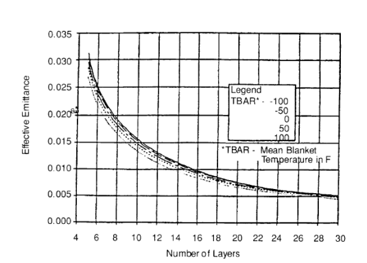The number of MLI layers is the only real design option that a thermal designer needs to address once he or she has determined that a blanket is needed for a given surface.  The effective emmitance of MLI blankets given the number of layers is shown in Figure 07, as taken from [Gilmore, 1994]. 

Figure 07: MLI Blanket Effective Emittance as taken from [Gilmore, 1994], pg. 4-79.

MLI blanketing will add about 0.73 kg/m² based on a 15 layer blanket.  Additionally, these blankets also provide a conductive path to the outer space environment.  While this is usually a small value as compared to the thermal radiation loss, this should be checked to be sure the MLI blankets do not provide too much conductive losses.  An estimate of the effective thermal conductivity of MLI blankets is given in [Gilmore, 1994] as the following equation (pg. 4-79), where the units of temperature are in Rankine.

 

 

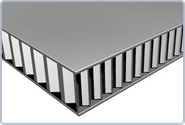
c.                   Radiator Panels are any surface dedicated to thermally communicate with the outside environment and serve as an interface between the internal components and the outside environment. Radiators typically are dedicated areas on the structure that serve to reject waste heat.  All radiators reject waste heat by IR thermal radiation and must reject not only the waste heat delivered to them, but also any absorbed heat loads gained from the environment.  The radiating power of a radiator depends on its emissivity and temperature.  Most radiators must have a high emissivity (>0.8) and a low absorbtivity (<0.2).  Typical finishes consists of silver or aluminized Teflon, paints with a low a/e, and quartz mirrors.  When a radiator is expected to be exposed to direct sunlight the use of Optical Solar Reflectors (OSR) is typically preferred.  These consist of small square mirrors that are highly reflective of ultraviolet radiation but also have a reasonable emissivity.  Sometimes the use of Flexible-OSRs (called FOSARS) when non-planar radiator surfaces are encountered.  

The radiators on most spacecraft orbiting the Earth are made from aluminum core honeycomb panels, which typically have a mass of 3.3 kg/m².  The unique feature of honeycomb panels is that they provide high strength at relatively low weights.  They also, have the unique characteristic of a very high through (inside to outside) thermal conductivity compared to their planar (spreading) thermal conductivity.  The relative value of these two thermal conductivities is somewhere around twenty.  This is due to the nature of their construction by adhesively attaching two very thin carbon graphite epoxy sheets that sandwich an aluminum honeycomb panel.  The aluminum honeycomb structure has a through conductivity value of around 3 to 10 W/m²K.  The carbon composite (CC) face sheets that are adhesively attached are usually very thin, in the order of 10 to 25 mils.  Since the type of honeycomb core can vary along with the face sheet thickness, typical values are misleading and the thermal engineer will have to inquire about their mechanical specifications.  After acquiring the face sheet materials and thickness’ a good estimate for the planar thermal conductivity is found by using the total thickness of both the face sheets along with the thermal conductivity of the material comprising the face sheets in the direction along their plane.  The through thickness can then be estimated using the following formula. The value of the through conductivity can be calculated using the following equation where the contribution from the adhesive layers can usually be ignored. 

 

Thin CC Face-Sheet

Al Honeycomb Core

Figure 08: Honeycomb Panel

The low thermal conductivity in the planar direction gives for a low spreading ability, which results in a low radiator panel effectiveness.  The radiator panel effectiveness is a concept similar to fin efficiency and is defined as the amount of heat radiated divided by the ideal amount of heat that could be radiated if the panel were at a uniform temperature.  Radiator panel effectiveness is a quantity that needs to be considered and is usually around 76% for honeycomb panels.  For a deployable radiator (extended panel radiator) with a base temperature of T_B whose both sides are exposed to a sink temperature of T_S and with an emissivity of e₁ and e₂, on each respective side, which also has embedded heat pipes spaced at distance of 2L, the estimated fin effectiveness as given by [Gilmore, 1994] on page 4-134 is shown here,

 

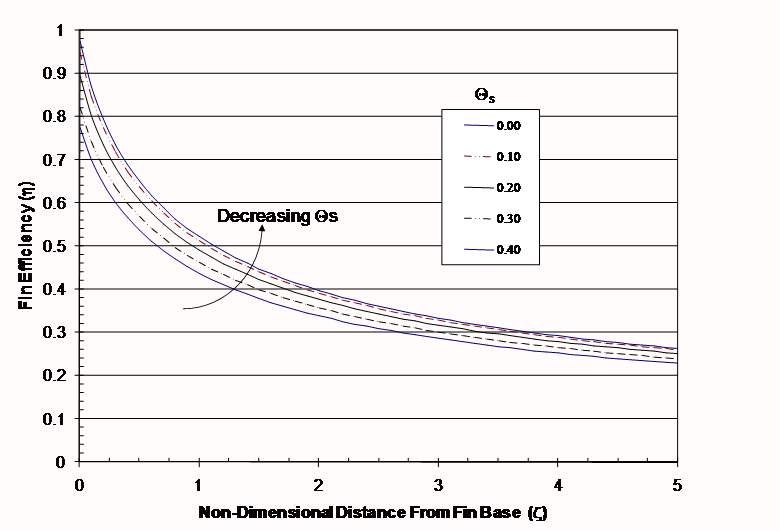
Where the fin thermal conductivity is given as k and the panel thickness is t.  For the case of a honeycomb panel that has two different thermal conductivity values (planar and through) the planar value should be used in the above equation.  Additionally, if the radiator panel is not an extended panel but radiates from one side only, [Harris & Simionescu, 2002] give the following graph for radiator panel effectiveness. 

Figure 09: Radiator Panel Effectiveness as taken from [Harris & Simionescu, 2002]

In Figure 09 above the following quantities were defined.

 

In addition, sometimes thermal conductive planes (called doublers) are attached to the inside surface of the radiator to increase the planer thermal conductivity of the honeycomb panel.  The use of doublers is usually needed to overcome a low radiator planar (spreading) thermal conductivity due to their thinness and are typically attached on the inside surface of the panel directly underneath a heat source.

Heaters & Thermostats – Ideally, heater power would not be necessary and a TCS will be completely passive.  However, this is seldom the case.  The large difference in the lunar environment between lunar day and lunar night will likely require some heater power usage during cold environmental conditions.  Heaters are also always included to provide backup heat when a component fails or is turned off and must be kept above a lower temperature limit.  However, the power usage by heaters must be kept to an absolute minimum since energy will be a precious commodity on any lunar system.  All heating systems will have manual overrides but will in most cases be controlled by some type of thermostat.  These can be either the bang-bang type or the proportional type.  The difference is that the latter type of thermostat allow for partial power being fed to the heating element instead of either fully on or fully off methods of operation (i.e. bang-bang).  The proportional type is usually preferred. While heater/thermostat systems add little mass and require a minimal volume claim, they always add complexity in the overall control logic and also add failure modes to the system.  All possible kinds of failures need to be accounted for (e.g. thermostat failed in the on position or the off position) and single point failure points must be eliminated.  Therefore, backup heaters and backup thermostats are the norm on most space deployed TCS. 

d.                  Thermal Louvers are another passive thermal control option.  They are essentially venetian blinds can be placed over any surface (unusually, thermal radiator panels) that automatically close as their temperature lowers and become fully open when their temperature rises above a set point.  Their benefit is that they provide a good view factor to the radiative heat sink when not needed and also can block the view to that sink under cold conditions.  Or, they are useful in blocking out solar radiation (shading) while allowing the radiator to ‘see’ its intended thermal radiation sink.  The mechanism that opens and closes the blinds is a bimetallic coil spring that can be designed to operate between two given temperature set points.  The design and other all engineering aspects of surrounding the design and operation of these devices are ignored here and only the necessary engineering performance data is highlighted for thermal control systems design.  Before describing their engineering performance characteristics it should be noted that these devices are expensive, bulky and add mass to the system.  It is suggested to add thermal louvers only when completely needed. They are a method of handling extreme cold environments when heaters will require too much energy.  Table 06 below [Gilmore, 1994] shows data from some flight qualified thermal louvers.  For thermal analysis purposes, a linear variation between the open and closed positions is assumed.  See equation below.  The emissivity is otherwise e_close for T < T_closed, and e_open for T > T_open. 

 

Table 06: Louver Effective Emissivity from Test Data, as taken from [Gilmore, 1994, pg. 4-106] Program Louver Size Radiator Hemispherical Emittance eeffective Tclosed Topen Radiator DT Open Closed ATS 45.7 x 58.2 cm OSR e=0.77 0.62 0.114 18 °C 32 °C 18 K ATS-6 45.7 x 58.2 cm Z-306 e=0.88 0.71 0.115 27.4 °C 32 °C 18.6 K GPS 40.6 x 40.5 cm Z-306 e=0.88 0.70 0.09     18 K Intelsat CRL 62.2 x 60.5 cm AgTEF e=0.76 0.67 0.08 20 °C 30 °C 10 K MMS Landsat-4 55.6 x 108.1 cm Z-306 e=0.88 0.39 0.10   15 °C 32 °C 17 K

The effective solar absorptance of a louvered panel is defined as the fraction of incident solar energy absorbed per unit area of the louvered surface.  The data on the effective solar absorbtivity is very scarce and is quite scattered.  However, the effective absorptance values published should inherently contain the effects of sun multireflection off specular components.  Figure 10 below [Gilmore, 1994] shows some test data on the solar absorptance variation with solar angles and blade angles.  An energy balance performed on the louvered radiator panel will yield the following equation.

Table 07: Flight-Qualified Rectangular-Blade Louver Assemblies, as taken from [Wertz & Larson, 1999], pg.443.    Orbital Sciences Corp. Swales & Assoc. Starsys No. of Blades 3 to 42 Various 1 to 16 Open Set Point (°C) Various 0 to 40 -20 to 50 Open/Close Differential (°C) 10 to 18 10 to 18 14 Dimensions (cm) Length Width Height   20 to 110 36 to 61 -   27 to 80 30 to 60 6.4   8 to 43 22 to 40 6.4 Area (m2) 0.07 to 0.6 0.08 to 0.5 0.02 to 0.2 Weight/Area (Kg/m2) 3.2 to 5.4 4.5 5.2 to 11.6

Additionally, [Wertz & Larson, 1999] give more data on available louver assemblies including dimensions and weights.  This data is shown below in Table 07.

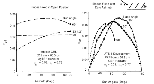
Figure 10: Louver Effective Solar Absorbtivity Variation with Azimuth and Blade Angle (test Data), taken from [Gilmore, 1994], pg. 4-108.

One note of caution is needed.  These devices are designed and used in the clean space environment.  Care of design will have to be exercised when using thermal louvers on the lunar surface due to the charged dust particles that will eventually inhibit any moving parts.  It is anticipated that any louvers that will be exposed to the lunar regolith will need to have all the moving surfaces sealed. 

 

e.                  Heat Pipes and Capillary Pump Loops - Heat pipes are common heat transport devices used to move heat up to several meters with little temperature drop along the pipe.  They essentially work through the means of phase change of an enclosed working fluid.  The working fluid is evaporated at the hot end of the heat pipe and then moves as a vapor to the cold end, whereby it condenses and is ‘pumped’ back to the evaporator by a wicked structure.  This evaporation/condensation cycle allows for heat transfer with a low associated temperature drop.  The devices are common both on earth based systems and in space borne systems.  They typically can transport from several watts up to hundreds watts of heat over distances of up to about a meter.  They are good devices to move heat from a device displaced from a radiator or cold plate when other means are unavailable.  They can also be embedded in radiator panels to increase the panel’s effectiveness.  However, space heat pipes are typically an aluminum/ammonia combination without a wick structure to pump the fluid to the evaporator.  They employ axially grooved aluminum pipes since there is no hydrostatic head to overcome in a zero gravity environment.  These pipes will generally not be applicable on the lunar surface.  Therefore, when using and specifying heat pipes for a lunar system it is suggested that wicked heat pipes be used that can work against a gravitational head.  Keep in mind that the lunar gravitational constant is about 1/6^th that of the Earth’s.  Also, water heat pipes will not be viable for any application where the temperature will approach the freezing point of water.  So, low freezing point fluids will have to be specified that are compatible with both the container and wick materials.  Finally, keep in mind that once a heat pipe is embedded in a system it should be understood that they are not thermal diodes.  A designer may decide to embed a heat pipe to help remove heat during the hot case only to learn that it increases the thermal losses during the cold case.  Therefore, caution is advised when using heat pipes.  There are diode heat pipes in use and a heat pipe specialist will need to be consulted to assist in the design and deployment of any heat pipes in a lunar TCS. 

Also used in space systems are a device called a capillary pump loop heat pipe (CPL).  These devices can move waste heat (in the vapor) over several tens of meters up to a hundred meters.  They also have been flight qualified for up to 2 kW.  However, they are expensive and temperamental devices that prefer steady state operation.  Also, the same caveat applies to these devices as was given for heat pipes.  That is. These devices have been designed for zero gravity environments.  Design modifications and qualification will be needed for any CPLs used on the lunar surface.  With that caution stated, heat pipes and CPLs offer a TCS designer a passive and highly reliable option for moving heat around in a system.  They should always be considered instead of moving heat through the use of a coolant pumped by a prime mover (such as a pump or fan).

5.                   Thermal Design Methodology is now described in a stepwise manner.  This procedure is to define how to indentify worst case lunar environmental temperatures based on the location on the Moon’s surface.  Once defined, these environmental temperatures are used to size and define radiator surface finishes.  Next, the operational temperatures under hot and cold extreme environments are found and cold case heater power requirements are reported.  We’ll explore this methodology step by step using an example computation.

a.                   Equivalent Environmental Temperatures are computed once the solar, albedo, and lunar surface IR loads are known based on the lunar latitude.  A heat balance is performed on every exposed surface using the equation below (which assumes a 0 K deep space temperature) once the surface finishes (a and e) are selected.  Worst case hot and cold extremes need to be identified for every surface, which depends on its orientation.  Therefore, it is recommended that the heat balance be performed for all four local lunar times: sunrise, noon, sunset, and midnight.  Once the F_solar and F_iew(view factor from the surface to the lunar surface) are found then T_env can be found.  This temperature represents an equivalent environmental radiative sink temperature for each particular surface. 

b.                  Radiator Operating Temperatures are next found using the equivalent environmental temperatures and the internal heating loads that need to be rejected (i.e. waste heat) that are supplied to the radiators.

It must be now be determined if the operating radiator temperature is acceptable, or if another surface finish, or more or less radiator area space claim is needed.  If so, then step a. needs to be repeated.  This iterative calculation needs to be repeated as many times as necessary to ensure that maximum operational temperatures can be assured by the radiator(s) design.  It also instructive at this point to compute the radiator surface effectiveness given the computed radiator temperatures, T_radiator.  The radiator temperature computed in the above equation is used as the fin base temperature T_B in the effectiveness relationships described in section 6.c.  Once the radiator effectiveness is found, then the actual radiator area needed will be found as follows.

Note, that most, if not all other surfaces will be blanketed and the outer blanket equivalent environmental temperatures should also be established during this iteration process.

c.                   Heater requirements are now computed based on worst case cold environments with the indentified (surface finish and area) radiator(s).  The heater power is found using the following formula. 

If the power required for the radiators is too high, then several option are available including the use of thermal louvers, or returning to step a. and redefining the radiator(s) surface area and or surface finish. 

d.                  Parasitic Heat Loss loads are finally found once all the exposed radiator(s) have been defined and maximum allowable operating temperate are verified not to be exceeded during worst case hot conditions, and the heater powers needed during worst case cold conditions are verified to lie within the allowable power budgets.  All other blanketed or otherwise protected surfaces will have parasitic heat losses during worst case cold extreme conditions and heater power may be necessary to ensure that survival temperatures are not violated.  Assuming that all protected surfaces are blanketed with MLI, then the final environmental temperatures found during the radiator design sequence for the MLI surfaces represents the outer layer temperature.  The parasitic heat losses are then found as follows.

Of course, the opposite may be a concern.  That is, the parasitic heat gains through the blanketed surfaces during worst case hot conditions may be too high.  This can also be easily found using the flowing equation.

6.                    Case Study of a Simple Geometry –As an example of the methodology laid-out in section 7. a simple six-sided box located at the lunar equator will be analyzed under worst case hot and cold conditions.  During these computations the surfaces best suited to act as the radiators will be analyzed, as determined by their respective orientations.  The six surfaces are defined as follows:

·         The nadir surface will be facing the lunar soil and assumed in direct thermal contact at all times

·         The opposite face is the zenith oriented face that looks away from the lunar surface at all times.  It, therefore, has no view of the lunar surface.  This face at times is exposed to direct sunlight, but never any albedo. 

·         The leading and trailing faces (east and west, respectively) always have a 50% view factor to the lunar surface and 50% view factor to space.  These two surfaces are at times exposed to direct and indirect sunlight (albedo).

·         The north and south oriented faces also have a 50 % view factor to the lunar surface and 50% view factor to space.  These two surfaces are at times exposed to reflected sunlight (albedo) but never direct sunlight due to the box being located at the lunar equator. 

Soil Temperatures Sunrise 90 K Noon 390 K Sunset 120 K Midnight 100   Hot Cold OSR e 0.8 0.8 a 0.12 0.08 MLI e 0.67 0.75 a 0.55 0.35

For the purposes of this example 8 mil Quartz OSRs will be used for thermal radiator surfaces and all other surfaces will be covered with 20 layered MLI blanketing.  The lunar soil temperatures and surface thermo-optical properties that will be used in this analysis are shown to the right.

For a sun facing surface (zenith oriented) Figure 02 shows that the incident solar fraction at lunar noon is 1.00. Therefore, this will represent the hot case for this surface. Also for the east and west oriented surfaces the solar fraction will also be 1.0 at the sunrise terminator (6:00 a.m. lunar time) and the sunset terminator(6:00 p.m. lunar time), respectively.  The north and south faces will never see direct solar energy sine the lunar location is at the equator. 

The resulting worst case hot and cold equivalent environmental temperatures for five of the side of the six-sided box are shown below in Table 08.  Looking at the results it appears that the north and south or east and west oriented faces are good candidates for the radiator surfaces.  This is because they have a lower temperature excursion (~225 K) between the hot and cold case extremes than does the zenith oriented face.  Although the zenith face has the lowest excursion temperature excursion for the cold case (213 K), it also has the lowest possible environmental temperature (that of space at 8 K) and would require the most amount of heater power during the cold case extremes.  But, there is a problem with not using the zenith face as the radiator  The worst case maximum temperatures for all other faces is 329 K, which is probably too high a radiator temperature for most electronics. . Therefore, we’ll use the zenith oriented face as the radiator and we may have to add thermal louvers if the heater requirements during cold conditions is too high. 

Therefore, we’ll use the zenith face as the radiator and blanket all other surfaces.  The next step will be to compute the radiator temperature when waste heat is being delivered to them.  Let’s assume that the maximum allowable radiator temperature is set at 40 °C. 

Table 08: Resulting Equivalent Environment Temperatures for Six-Sided Geometry at Lunar Equator [K] Sunrise Noon Sunset Midnight Max Min Excursion Zenith hot 8 245 8 8 245 8 237 cold 8 221 8 8 221 8 213 North hot 113 329 124 116 329 113 216 cold 104 329 117 108 329 104 225 East hot 247 329 124 116 329 116 213 cold 224 329 117 108 329 108 218 West hot 113 329 248 116 329 113 216 cold 104 329 225 108 329 104 225 South hot 113 329 124 116 329 113 216 cold 104 329 117 108 329 104 225

Therefore, the maximum power flux that the zenith radiator surface could accommodate is as follows.

This value appears low and if the box needed to reject larger quantities of heat a deployable radiator may be needed.  Also, keep in mind that including the radiator effectiveness, of say 76%, then the maximum amount of waste heat that could be rejected at 40 °C is 206.7 W/m². 

Let’s continue, however, and compute the heater power that would be needed during the worst case cold environment when all internal components are off.  We’ll use a radiator minimum survival temperature of -15 °C. 

There is a problem here in that we need almost as much heater power in the cold case as the waste heat generated in the system.  And this is even before adjusting for radiator panel effectiveness.  Let’s place thermal louvers over the radiator and recomputed the maximum power that can be rejected at 40 °C during the hot case and the heater power required to keep the radiator at -15 °C during the cold case.  We’ll use a value of emissivity for the louvers of 0.7 when fully open and 0.09 when fully closed. 

Table 09: parasitic heat losses through MLI blanketed surfaces at lunar midnight for internal surfaces at 300 K. Surface Min [K] Qloss[W/m2] Nadir 100 3.6 North 144 3.5 East 146 3.5 West 144 3.5 South 144 3.5 Total 17.5

Finally, let’s compute the parasitic heat losses off the other five sides during the worst case cold conditions.  For this final analysis we’ll use an effective thermal conductivity of 0.008 (20 layers) as the value for the emissivity through the MLI blanketing to the equivalent environmental temperatures.  For the soil facing surface (nadir) the environmental temperature used will be the soil temperature. 

7.                   Concluding Remark and Final Thoughts - A few final comments regarding the use of commercial software are in order.  The methods described here are for top level hand calculations in order to establish some baseline parameters regarding any TCS designed to accomplish lunar mission goals.  Only the very simplest of geometries can be analyzed without the use of commercial software due to the geometrical complexities related to radiative heat exchanges and associated external environmental loads.  While there are several very powerful software packages available for thermal engineering, care was taken not to mention any.  A quick internet search on satellite thermal software will produce the products most used by thermal engineers at NASA and other aerospace companies.  Most of these are based upon older FORTRAN programs developed under NASA in the 1970’s and 1980’s.  Most of these FOTRAN codes were developed during the era of field delimited input files (decks) that contained data in field specified formats.  These codes are SINDA (a thermal analyzer) and TRASYS (a radiative analyzer) and form the kernel for some modern windows based and highly GUI software packages.  Also, a nice feature of several of these software packages is the ease at which orbital environmental loads are generated and fed directly into the thermal analyzer.   While, both SINDA and TRASYS are public domain software, they require a FORTRAN compiler to execute.  Support for the FORTRAN versions of these programs has waned over the last decade and are difficult to run under Microsoft Visual FORTAN (10.0 is the latest version released at the time this handbook was written).  The versions most commonly found that are free and unsupported need DEC (or later Compaq) Visual FORTRAN v. 6 to run.  Therefore, for a more complete, accurate, and professional thermal analysis and design a newer thermal software package will need to be acquired at around several thousand dollars for a single seat license. 

 

8.                   References

Eckart, Peter, 2006, The Lunar Base Handbook, 2^nd Ed., McGraw-Hill, ISBN 978-0-07-329444-5.

Gilmore, David G., 1994, Satellite Thermal Control Handbook, The Aerospace Corporation Press, El Segundo, CA, ISBN 1-884989-00-4.

Harris, Daniel K. & Simionescu, Florentina, 2002, “Radiating Fin Analysis Using an Extended Perturbation Series Solution Technique,” J. Spacecraft, v 40(1), pp. 141-142. 

Henninger, John, H., 1984, “Solar Absorptance and Thermal Emmitance of Some Common Spacecraft Thermal-Control Coatings,” NASA Reference Publication 1121.

Modest, Michael F., 1993, Radiative Heat Transfer, McGraw-Hill, ISBN 0-07-042675-9.

Wertz, James R. & Larson, Wiley J., 1999, Space Mission Analysis, 3^rd Ed. Microcosm Press, ISBN 978-1-881883-10-4.

 

---