6. Velocity Saturation Effect Experiments (45nm - 2um)
6.1. Objectives
- set up your .bashrc to use Sentaurus tools 2011.9
- learn how to load in Sentaurus Work Bench (swb) Project
- learn how to use swb
- examine effect of velocity saturation on Ids-Vds, Vdsat, Idsat
- better understand what happens beyond “saturation”
6.2. Required Programs
- sde
- sdevice
- tecplot_sv
- inspect
- swb
6.3. Overview
See lecture notes on 3-terminal and 4-terminal MOS devices.
6.4. Getting the files
First, log on to niu003.eng.auburn.edu.
Then in a command terminal, run
cd
This ensures you will change to home directory. Then, run
/scratch/getfiles.sh
This will copy a file physics.gzp to your home folder, and update your .bashrc so that you can now use the Sep 2011 version of the tcad tools.
As this is an existing window, we need to source the .bashrc file. Just run
source .bashrc
To launch swb, run
swb
6.5. Loading in a swb project
To load in the physics.gzp project, first look for the file physics.gzp as shown below in swb’s file browser:

Figure 1: locate project archive
Right click the file, select open, you should see:
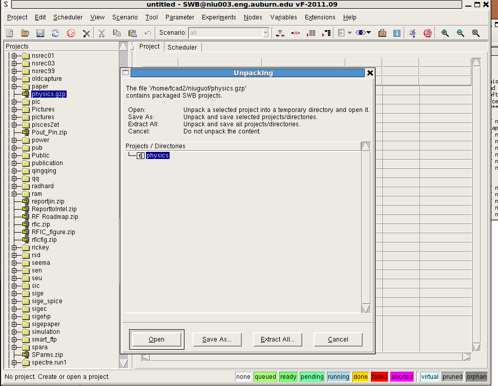
Figure 2: extract project archive
Select extract all, then create new folder or just use default to place the project.
Wait a little while. It is about 25 MB zipped, so big. You shall see:

Figure 3: Velocity Saturation Physics swb project
You are now in a position to examine the impact of vsat. You can check out the Vds dependence, Lg dependence, etc. You can also on the command line look at the plt and tdr files produced. You can use tecplot_sv to look at those as well.
To save your disk space, I have commented out the commands for saving .tdr files during Vd sweep. There, however, is still at least one tdr file, which is saved in the very end, that is, for the highest Vgs and Vds. Check your folder, sort it by date, you will see which files are new.
6.6. Mesh
Always examine your structure and mesh before running a lot of simulations. A sample mesh for the 65nm device is shown below:

Figure 4: 65nm device mesh.
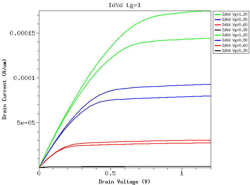
6.7. Id-Vd Curves
The Id-Vd curves for each gate length obtained with and without turning on velocity saturation effect are overlayed, so that we can see the impact of velocity saturation directly.
Simulations were run for all the gate length from 45nm to 2um, which produce the following Id-Vd plots:
6.7.1. 2um
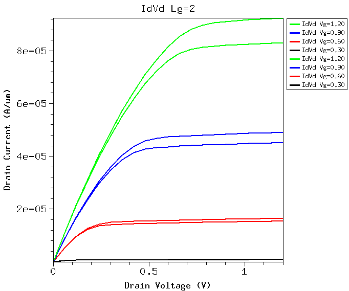
Figure 5: Id-Vd, lgate = 2um.
There is visible but small difference for 2um gate length.
6.7.3. 0.5um or 500nm
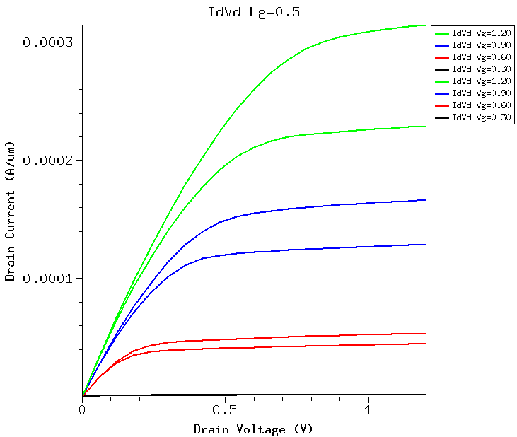
Figure 7: Id-Vd, lgate = 0.5um.
Vsat makes much more difference.
Id is smaller, and Vdsat is smaller too, as expected.
Velocity saturation occurs at a smaller Vd than drain end channel pinch-off, therefore, Id starts to saturate earlier with velocity saturation.
Now pay attention to the Vds at which saturation starts to occur, or Vdsat, for the same gate voltage as gate length varies further.
6.7.4. 0.35um or 350nm
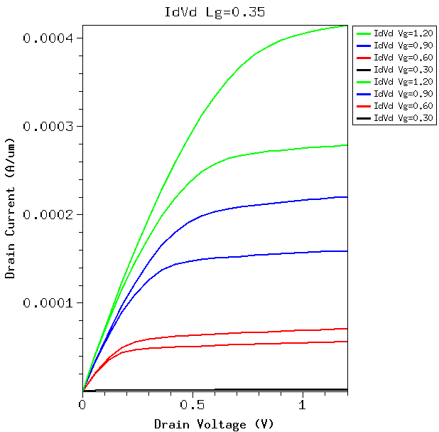
Figure 8: Id-Vd, lgate = 0.35um.
6.7.5. 0.18um or 180nm
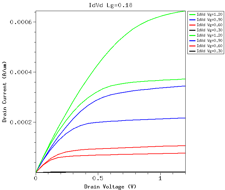
Figure 9: Id-Vd, lgate = 0.18um.
6.7.6. 0.13um or 130nm
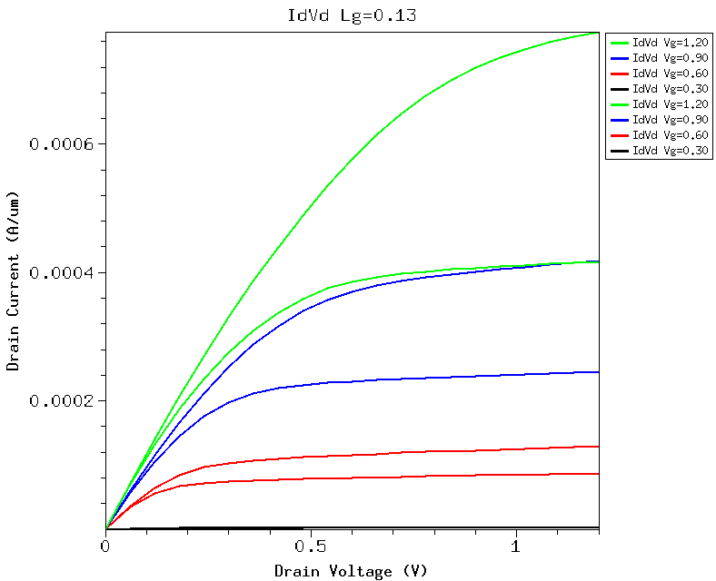
Figure 10: Id-Vd, lgate = 0.13um.
6.7.7. 0.065um or 65nm
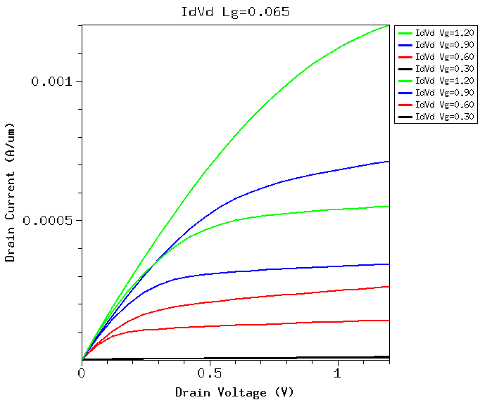
Figure 11: Id-Vd, lgate = 65nm.
Now you can summarize how the impact of velocity saturation changes with gate length. Think about these questions:
- Does the impact on Idsat and Vdsat become stronger with gate length scaling?
- For the same gate length, why is the effect stronger at higher Vd?
- For the same high Vd = Vdd, at the same lgate, is the impact on Id stronger at higher Vg or lower Vg? Why? Consider only the higher Vg values (above threshold), when the channel is inverted. This is a pretty challenging question without a simple answer. But I encourage you to think about it, and try to make some observations.
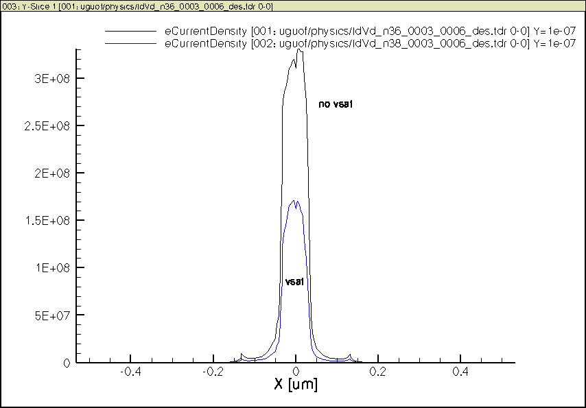
6.8. Lateral field and Velocity at Mid Channel Point
Velocity saturation is a high lateral field effect. So let us look at how the lateral field in the channel varies with Vd. You should turn on the tdr file saving to see position dependence. Below are some mid channel point plots made using the CurrentPlot technique.
6.8.1. 2um
6.8.1.1. Lateral field and eVelocity
The lateral field at mid channel for 2um lgate is shown below:

Figure 12: Ex at mid channel point at surface versus Vd, lgate = 2um.
The corresponding eVelocity is:

Figure 13: eVelocity at mid channel point at surface versus Vd, lgate = 2um.
Pretty much at lower Vds, the channel is like a resistor, varying Vg simpy changes resistance, but the lateral field is simply Vds/L, and thus indpendent of Vg.
The difference is at high Vd, when saturation occurs. With velocity saturation, drain current saturation occurs at a smaller Vd, which will then make the Ex inside the channel saturate too. Recall much of the extra Vd beyond saturation will be drop over a very narrow region near the drain.
After saturation occurs, the intrinsic channel’s surface potential and hence lateral electric field will no longer change much. This means the mid channel lateral field Ex will also stay pretty much saturated.
Think about these plots and see if they make intuitive sense to you. For 2um lgate, velocity saturation plays little role. It is pretty much showing classic long channel behavior.
6.8.1.2. Velocity Saturation Region
This high field region near the drain used to be called “pinch-off” region. As velocity saturation is a fact of life for these short channel devices, and velocity saturation occurs before pinch-off, this high field region near the drain is more properly called velocity saturation region (VSR).
6.8.1.3. eVelocity vs Ex
Can you think about why the Ex plot does not have exactly the same shape as the eVelocity plot? Hint: think about mobility and how mobility changes with increasing Vg.
Note
Answer: The decrease of mobility with increasing Vg (recall the surface roughness effect, and the Enormal dependence we investigated earlier) caused this difference.
See also if you can correlate the velocity plot to the Id-Vd plot shown above for 2um. Does it make sense to you?
The eVelocity in the linear operation region is clearly higher for lower Vgs, but Id in the linear region is still higher for higher Vgs, can you think of a possible reason?
Note
Inversion charge density increases with increasing Vg. This increase dominates over the decrease of eVelocity, so the net result is still increase of drain current with increasing gate voltage.
6.8.2. 65nm
At 2um, velocity saturation is not significant for most part of the channel, if you use tecplot_sv to look at the velocity vs x plot.
Let us look at the mid channel point.
6.8.2.1. eVelocity at Mid Channel

Figure 14: eVelocity at mid channel point at surface versus Vd, lgate = 65nm.
We now clearly see the strong impact of velocity saturation on the electron velocity at mid channel point, that is, velocity at higher Vds is much reduced with velocity saturation compared to without velocity saturation.
If we repeat the plots for other gate lengths, as we did for Id-Vd above, we find that mid channel velocity is affected more for shorter gate lengths. At 65nm, there is much more difference.
6.8.2.2. Ex at Mid Channel
Note that velocity saturation effect also has caused change of the e-field as well, so you cannot simply assume E will be the same when you turn on velocity saturation effect. It is a self consistent solution of all equations in the end.
The Ex at mid channel at surface versus Vd for 65nm is shown below:

Figure 15: Ex at mid channel point at surface versus Vd, lgate = 65nm.
6.9. Inspecting Internal Details
Much of the above analysis is about the mid channel point. Ideally you always want to probe the 2D distribution of internal physical quanities, such as potential, eDensity, eVelocity etc.
Comparing 2D plots, e.g. eDensity distribution between with and without vsat, however, can be challenging. You can put them side by side, and observe their differences.
Ideally you want to “overlay” them, this is impossible if we make contour plots. We might make 3D surface plots instead of 2D countour plots. Even this can be hard.
For MOSFETs, a particular 1-D cut of the y-axis at the Si surface, can be used instead. Essentially this shows a cut along the channel from source to drain.
We can load in the .tdr files corresponding to the same Vg and Vd, simulated with and without vsat effect, make y-cut at the surface, then compare about everything we are interested in.
We have in fact made reference to insights gained from such 1D cuts. A number of plots are given below to assist understanding.
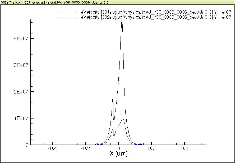
6.9.1. 2um (long channel)
6.9.1.1. Surface potential

Figure 16: Surface potential along channel, lgate = 2um.
6.9.1.2. Surface eVelocity

Figure 17: Surface evelocity along channel, lgate = 2um.
6.9.1.3. Other Plots
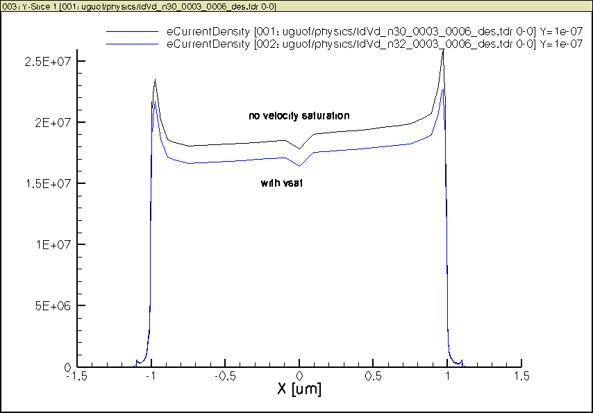
Figure 18: Jn along channel, lgate = 2um.
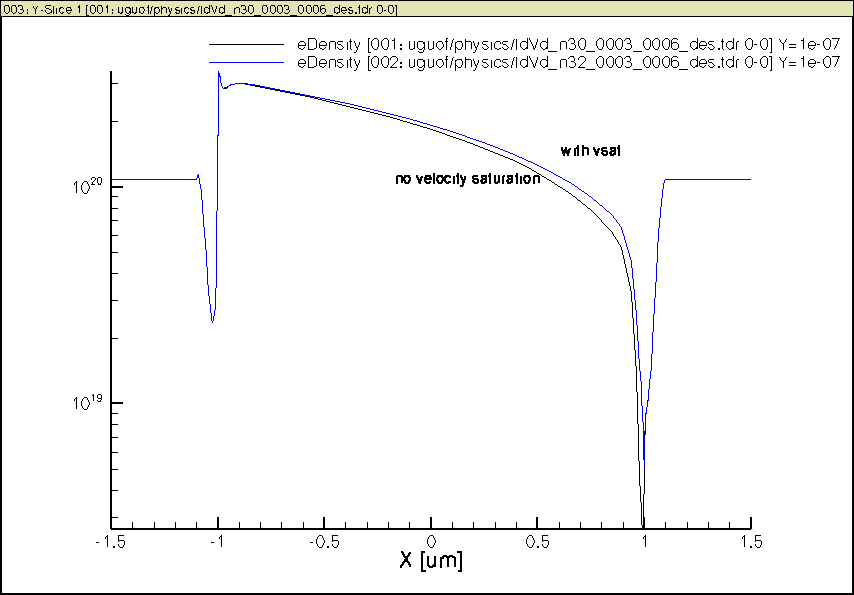
Figure 19: Surface n along channel, lgate = 2um.
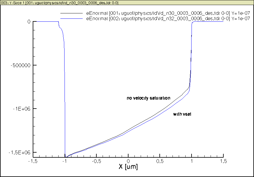
Figure 20: E-field normal to current flow along channel, lgate = 2um.
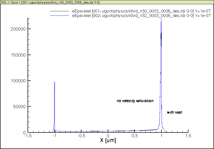
Figure 21: E-field parallel to current flow along channel, lgate = 2um.

6.10. Homework
Play with the swb project, save graphics, and write up any analysis you come up on the impact of velocity saturation, e.g. dependence on Lg, Vd, Vg. You can look at internal velocity too, even the .tdr files.
This will get you ready for our mid term project.