Note:
The chapter describes functions for image processing and analysis.
Most of the functions work with 2d arrays of pixels. We refer the arrays
as "images" however they do not neccesserily have to be IplImage's, they may
be CvMat's or CvMatND's as well.
Drawing functions work with arbitrary 8-bit images or single-channel images
with larger depth: 16s, 32s, 32f, 64f
All the functions include parameter color that means rgb value (that may be
constructed with CV_RGB macro) for color images and brightness
for grayscale images.
If a drawn figure is partially or completely outside the image, it is clipped.
Constructs a color value
#define CV_RGB( r, g, b ) (int)((uchar)(b) + ((uchar)(g) << 8) + ((uchar)(r) << 16))
Draws simple or thick line segment
void cvLine( CvArr* img, CvPoint pt1, CvPoint pt2, double color, int thickness=1, int connectivity=8 );
The function cvLine draws the line segment between pt1 and pt2 points in the
image. The line is clipped by the image or ROI rectangle. The 8-connected or 4-connected Bresenham
algorithm is used for simple line segments. Thick lines are drawn with rounding
endings. To specify the line color, the user may use the macro CV_RGB( r, g, b ).
Draws antialiased line segment
void cvLineAA( CvArr* img, CvPoint pt1, CvPoint pt2, double color, int scale=0 );
The function cvLineAA draws the 8-connected line segment between pt1 and pt2
points in the image. The line is clipped by the image or ROI rectangle. The algorithm
includes some sort of Gaussian filtering to get a smooth picture. To specify the
line color, the user may use the macro CV_RGB( r, g, b ).
Draws simple, thick or filled rectangle
void cvRectangle( CvArr* img, CvPoint pt1, CvPoint pt2, double color, int thickness=1 );
The function cvRectangle draws a rectangle with
two opposite corners pt1 and pt2.
Draws simple, thick or filled circle
void cvCircle( CvArr* img, CvPoint center, int radius, double color, int thickness=1 );
The function cvCircle draws a simple or filled circle with given center and
radius. The circle is clipped by ROI rectangle. The Bresenham algorithm is used
both for simple and filled circles. To specify the circle color, the user may
use the macro CV_RGB ( r, g, b ).
Draws simple or thick elliptic arc or fills ellipse sector
void cvEllipse( CvArr* img, CvPoint center, CvSize axes, double angle,
                double startAngle, double endAngle, double color, int thickness=1 );
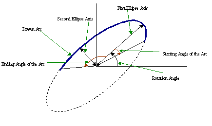
The function cvEllipse draws a simple or thick elliptic arc or fills an ellipse sector. The arc is clipped by ROI rectangle. The generalized Bresenham algorithm for conic section is used for simple elliptic arcs here, and piecewise-linear approximation is used for antialiased arcs and thick arcs. All the angles are given in degrees. The picture below explains the meaning of the parameters.
Parameters of Elliptic Arc
Draws antialiased elliptic arc
void cvEllipseAA( CvArr* img, CvPoint center, CvSize axes, double angle,
                  double startAngle, double endAngle, double color, int scale=0 );
The function cvEllipseAA draws an antialiased elliptic arc. The arc is clipped by ROI rectangle. The generalized Bresenham algorithm for conic section is used for simple elliptic arcs here, and piecewise-linear approximation is used for antialiased arcs and thick arcs. All the angles are in degrees.
Fills polygons interior
void cvFillPoly( CvArr* img, CvPoint** pts, int* npts, int contours, double color );
The function cvFillPoly fills an area bounded by several polygonal contours. The function fills complex areas, for example, areas with holes, contour self-intersection, etc.
Fills convex polygon
void cvFillConvexPoly( CvArr* img, CvPoint* pts, int npts, double color );
The function cvFillConvexPoly fills convex polygon interior. This function is much faster than the function cvFillPoly and fills not only the convex polygon but any monotonic polygon, that is, a polygon whose contour intersects every horizontal line (scan line) twice at the most.
Draws simple or thick polygons
void cvPolyLine( CvArr* img, CvPoint** pts, int* npts, int contours, int isClosed,
                 double color, int thickness=1, int connectivity=8 );
The function cvPolyLine draws a set of simple or thick polylines.
Draws antialiased polygons
void cvPolyLineAA( CvArr* img, CvPoint** pts, int* npts, int contours,
                   int isClosed, int color, int scale =0);
The function cvPolyLineAA draws a set of antialiased polylines.
Initializes font structure
void cvInitFont( CvFont* font, CvFontFace fontFace, float hscale,
                 float vscale, float italicScale, int thickness );
CV_FONT_VECTOR0 is currently
supported.
1.0f, the characters have the original
width depending on the font type. If equal to 0.5f, the characters are of half
the original width.
1.0f, the characters have the original
height depending on the font type. If equal to 0.5f, the characters are of half
the original height.
1.0f means ≈45° slope, etc.
thickness Thickness of lines composing letters outlines. The function cvLine is
used for drawing letters.
The function cvInitFont initializes the font structure that can be passed further into text drawing functions. Although only one font is supported, it is possible to get different font flavors by varying the scale parameters, slope, and thickness.
Draws text string
void cvPutText( CvArr* img, const char* text, CvPoint org, CvFont* font, int color );
The function cvPutText renders the text in the image with the specified font and color. The printed text is clipped by ROI rectangle. Symbols that do not belong to the specified font are replaced with the rectangle symbol.
Retrieves width and height of text string
void cvGetTextSize( CvFont* font, const char* textString, CvSize* textSize, int* ymin );
The function cvGetTextSize calculates the binding rectangle for the given text string when a specified font is used.
Calculates first, second, third or mixed image derivatives using extended Sobel operator
void cvSobel( const CvArr* I, CvArr* J, int dx, int dy, int apertureSize=3 );
apertureSize=1 3x1 or 1x3 kernel is used (Gaussian smoothing is not done).
There is also special value CV_SCHARR (=-1) that corresponds to 3x3 Scharr filter that may
give more accurate results than 3x3 Sobel. Scharr aperture is:
| -3 0  3|
|-10 0 10|
| -3 0  3|
for x-derivative or transposed for y-derivative.
The function cvSobel calculates the image derivative by convolving the image with the appropriate kernel:
J(x,y) = dox+oyI/dxox•dyoy |(x,y)The Sobel operators combine Gaussian smoothing and differentiation so the result is more or less robust to the noise. Most often, the function is called with (ox=1, oy=0, apertureSize=3) or (ox=0, oy=1, apertureSize=3) to calculate first x- or y- image derivative. The first case corresponds to
  |-1  0  1|
  |-2  0  2|
  |-1  0  1|
kernel and the second one corresponds to
  |-1 -2 -1|
  | 0  0  0|
  | 1  2  1|
or
  | 1  2  1|
  | 0  0  0|
  |-1 -2 -1|
kernel, depending on the image origin (
origin field of IplImage structure).
No scaling is done, so the destination image usually has larger by absolute value numbers than
the source image. To avoid overflow, the function requires 16-bit destination image if
the source image is 8-bit. The result can be converted back to 8-bit using cvConvertScale or
cvConvertScaleAbs functions. Besides 8-bit images the function can process 32-bit floating-point
images. Both source and destination must be single-channel images of equal size or ROI size.
Calculates Laplacian of the image
void cvLaplace( const CvArr* I, CvArr* J, int apertureSize=3 );
The function cvLaplace calculates Laplacian of the source image by summing second x- and y- derivatives calcualted using Sobel operator:
J(x,y) = d2I/dx2 + d2I/dy2
Specifying apertureSize=1 gives the fastest variant that is equal to
convolving the image with the following kernel:
|0  1  0|
|1 -4  1|
|0  1  0|
As well as in cvSobel function, no scaling is done and the same combinations of input and output formats are supported.
Implements Canny algorithm for edge detection
void cvCanny( const CvArr* img, CvArr* edges, double threshold1,
              double threshold2, int apertureSize=3 );
The function cvCanny finds the edges on the input image img and marks them in the
output image edges using the Canny algorithm. The smallest of threshold1 and
threshold2 is used for edge linking, the largest - to find initial segments of strong edges.
Calculates two constraint images for corner detection
void cvPreCornerDetect( const CvArr* img, CvArr* corners, int apertureSize=3 );
The function cvPreCornerDetect finds the corners on the input image img and stores
them in the corners image in accordance with Method 1 for corner detection desctibed
in the guide.
Calculates eigenvalues and eigenvectors of image blocks for corner detection
void cvCornerEigenValsAndVecs( const CvArr* I, CvArr* eigenvv,
                               int blockSize, int apertureSize=3 );
For every pixel the function cvCornerEigenValsAndVecs considers
blockSize × blockSize neigborhood S(p). It calcualtes
covariation matrix of derivatives over the neigborhood as:
    | sumS(p)(dI/dx)2   sumS(p)(dI/dx•dI/dy)|
M = |                                 |
    | sumS(p)(dI/dx•dI/dy)  sumS(p)(dI/dy)2 |
After that it finds eigenvectors and eigenvalues of the resultant matrix and stores
them into destination image in form
(λ1, λ2, x1, y1, x2, y2),
where
λ1, λ2 - eigenvalues of M; not sorted
(x1, y1) - eigenvector corresponding to λ1
(x2, y2) - eigenvector corresponding to λ2
Calculates minimal eigenvalue of image blocks for corner detection
void cvCornerMinEigenVal( const CvArr* img, CvArr* eigenvv, int blockSize, int apertureSize=3 );
img
The function cvCornerMinEigenVal is similar to cvCornerEigenValsAndVecs but it calculates and stores only the minimal eigen value of derivative covariation matrix for every pixel, i.e. min(λ1, λ2) in terms of the previous function.
Refines corner locations
void cvFindCornerSubPix( IplImage* I, CvPoint2D32f* corners,
                         int count, CvSize win, CvSize zeroZone,
                         CvTermCriteria criteria );
win=(5,5) then
5*2+1 × 5*2+1 = 11 × 11 search window is used.
criteria may specify either of or both the maximum
number of iteration and the required accuracy.
The function cvFindCornerSubPix iterates to find the sub-pixel accurate location of a corner, or "radial saddle point", as shown in on the picture below.
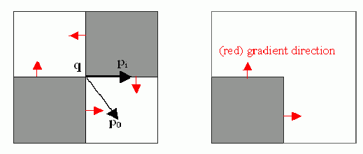
Sub-pixel accurate corner (radial saddle point) locator is based on the
observation that any vector from q to p is orthogonal to the image gradient.
The core idea of this algorithm is based on the observation that every vector
from the center q to a point p located within a neighborhood of q is orthogonal
to the image gradient at p subject to image and measurement noise. Thus:
εi=DIpiT•(q-pi)where
DIpi is the image gradient
at the one of the points pi in a neighborhood of q .
The value of q is to be found such that εi is minimized.
A system of equations may be set up with εi' set to zero:
sumi(DIpi•DIpiT)•q - sumi(DIpi•DIpiT•pi) = 0
where the gradients are summed within a neighborhood ("search window") of q.
Calling the first gradient term G and the second gradient term b gives:
q=G-1•b
The algorithm sets the center of the neighborhood window at this new center q
and then iterates until the center keeps within a set threshold.
Determines strong corners on image
void cvGoodFeaturesToTrack( IplImage* image, IplImage* eigImage, IplImage* tempImage,
                            CvPoint2D32f* corners, int* cornerCount,
                            double qualityLevel, double minDistance );
image.
eigImage.
The function cvGoodFeaturesToTrack finds corners with big eigenvalues in the
image. The function first calculates the minimal eigenvalue for every source image pixel
using cvCornerMinEigenVal function and stores them in eigImage.
Then it performs non-maxima suppression (only local maxima in 3x3 neighborhood remain).
The next step is rejecting the corners with the
minimal eigenvalue less than qualityLevel•max(eigImage(x,y)). Finally,
the function ensures that all the corners found are distanced enough from one
another by considering the corners (the most strongest corners are considered first)
and checking that the distance between the newly considered feature and the features considered earlier
is larger than minDistance. So, the function removes the features than are too close
to the stronger features.
Initializes line iterator
int cvInitLineIterator( const CvArr* img, CvPoint pt1, CvPoint pt2,
                        CvLineIterator* lineIterator, int connectivity=8 );
The function cvInitLineIterator initializes the line iterator and returns the
number of pixels between two end points. Both points must be inside the image.
After the iterator has been initialized, all the points on the raster line that
connects the two ending points may be retrieved by successive calls of
CV_NEXT_LINE_POINT point. The points on the line are calculated one by one using
4-connected or 8-connected Bresenham algorithm.
    CvScalar sum_line_pixels( IplImage* img, CvPoint pt1, CvPoint pt2 )
    {
        CvLineIterator iterator;
        int blue_sum = 0, green_sum = 0, red_sum = 0;
        int count = cvInitLineIterator( img, pt1, pt2, &iterator, 8 );

        for( int i = 0; i < count; i++ ){
            blue_sum += iterator.ptr[0];
            green_sum += iterator.ptr[1];
            red_sum += iterator.ptr[2];
            CV_NEXT_LINE_POINT(iterator);

            /* print the pixel coordinates: demonstrates how to calculate the coordinates */
            {
            int offset, x, y;
            /* assume that ROI is not set, otherwise need to take it into account. */
            offset = iterator.ptr - (uchar*)(img->imageData);
            y = offset/img->widthStep;
            x = (offset - y*img->widthStep)/(3*sizeof(uchar) /* size of pixel */);
            printf("(%d,%d)\n", x, y );
            }
        }
        return cvScalar( blue_sum, green_sum, red_sum );
    }
Reads raster line to buffer
int cvSampleLine( const CvArr* img, CvPoint pt1, CvPoint pt2,
                  void* buffer, int connectivity=8 );
pt2.x-pt1.x|+1, |pt2.y-pt1.y|+1 ) points in case
of 8-connected line and |pt2.x-pt1.x|+|pt2.y-pt1.y|+1 in case
of 4-connected line.
The function cvSampleLine implements a particular case of application of line
iterators. The function reads all the image points lying on the line between pt1
and pt2, including the ending points, and stores them into the buffer.
Retrieves pixel rectangle from image with sub-pixel accuracy
void cvGetRectSubPix( const CvArr* I, CvArr* J, CvPoint2D32f center );
The function cvGetRectSubPix extracts pixels from I:
J( x+width(J)/2, y+height(J)/2 )=I( x+center.x, y+center.y )
where the values of pixels at non-integer coordinates ( x+center.x, y+center.y ) are retrieved using bilinear interpolation. Every channel of multiple-channel images is processed independently. Whereas the rectangle center must be inside the image, the whole rectangle may be partially occluded. In this case, the replication border mode is used to get pixel values beyond the image boundaries.
Retrieves pixel quadrangle from image with sub-pixel accuracy
void cvGetQuadrangeSubPix( const CvArr* I, CvArr* J, const CvArr* M,
                           int fillOutliers=0, CvScalar fillValue=cvScalarAll(0) );
A|b] (see the discussion).
fillOutliers=0) or set them a fixed value (fillOutliers=1).
fillOutliers=1.
The function cvGetQuadrangleSubPix extracts pixels from I at sub-pixel accuracy
and stores them to J as follows:
J( x+width(J)/2, y+height(J)/2 )= I( A11x+A12y+b1, A21x+A22y+b2 ), whereAandbare taken fromM| A11 A12 b1 | M = | | | A21 A22 b2 |
where the values of pixels at non-integer coordinates A•(x,y)T+b are retrieved using bilinear interpolation. Every channel of multiple-channel images is processed independently.
#include "cv.h"
#include "highgui.h"
#include "math.h"

int main( int argc, char** argv )
{
    IplImage* src;
    /* the first command line parameter must be image file name */
    if( argc==2 && (src = cvLoadImage(argv[1], -1))!=0)
    {
        IplImage* dst = cvCloneImage( src );
        int delta = 1;
        int angle = 0;

        cvNamedWindow( "src", 1 );
        cvShowImage( "src", src );

        for(;;)
        {
            float m[6];
            double factor = (cos(angle*CV_PI/180.) + 1.1)*3;
            CvMat M = cvMat( 2, 3, CV_32F, m );
            int w = src->width;
            int h = src->height;

            m[0] = (float)(factor*cos(-angle*2*CV_PI/180.));
            m[1] = (float)(factor*sin(-angle*2*CV_PI/180.));
            m[2] = w*0.5f;
            m[3] = -m[1];
            m[4] = m[0];
            m[5] = h*0.5f;

            cvGetQuadrangleSubPix( src, dst, &M, 1, cvScalarAll(0));

            cvNamedWindow( "dst", 1 );
            cvShowImage( "dst", dst );

            if( cvWaitKey(5) == 27 )
                break;

            angle = (angle + delta) % 360;
        }
    }
    return 0;
}
Resizes image
void cvResize( const CvArr* I, CvArr* J, int interpolation=CV_INTER_LINEAR );
The function cvResize resizes image I so that it fits exactly to J.
If ROI is set, the function consideres the ROI as supported as usual.
the source image using the specified structuring element B
that determines the shape of a pixel neighborhood over which the minimum is taken:
C=erode(A,B): C(I)=min(K in BI)A(K)
The function supports the in-place mode when
the source and destination pointers are the same. Erosion can be applied several
times iterations parameter. Erosion on a color image means independent
transformation of all the channels.
Creates structuring element
IplConvKernel* cvCreateStructuringElementEx( int nCols, int nRows, int anchorX, int anchorY,
                                             CvElementShape shape, int* values );
CV_SHAPE_RECT , a rectangular element;
CV_SHAPE_CROSS , a cross-shaped element;
CV_SHAPE_ELLIPSE , an elliptic element;
CV_SHAPE_CUSTOM , a user-defined element. In this case the parameter values
specifies the mask, that is, which neighbors of the pixel must be considered.
NULL , then all values are considered
non-zero, that is, the element is of a rectangular shape. This parameter is
considered only if the shape is CV_SHAPE_CUSTOM .
The function cv CreateStructuringElementEx allocates and fills the structure
IplConvKernel , which can be used as a structuring element in the morphological
operations.
Deletes structuring element
void cvReleaseStructuringElement( IplConvKernel** ppElement );
The function cv ReleaseStructuringElement releases the structure IplConvKernel that
is no longer needed. If *ppElement is NULL , the function has no effect. The
function returns created structuring element.
Erodes image by using arbitrary structuring element
void cvErode( const CvArr* A, CvArr* C, IplConvKernel* B=0, int iterations=1 );
NULL, a 3×3 rectangular
structuring element is used.
The function cvErode erodes the source image using the specified structuring element B that determines the shape of a pixel neighborhood over which the minimum is taken:
C=erode(A,B): C(x,y)=min((x',y') in B(x,y))A(x',y')
The function supports the in-place mode when
the source and destination pointers are the same. Erosion can be applied several
times iterations parameter. Erosion on a color image means independent
transformation of all the channels.
Dilates image by using arbitrary structuring element
void cvDilate( const CvArr* A, CvArr* C, IplConvKernel* B=0, int iterations=1 );
NULL, a 3×3 rectangular
structuring element is used.
The function cvDilate dilates the source image using the specified structuring element B that determines the shape of a pixel neighborhood over which the maximum is taken:
C=dilate(A,B): C(x,y)=max((x',y') in B(x,y))A(x',y')
The function supports the in-place mode when
the source and destination pointers are the same. Dilation can be applied several
times iterations parameter. Dilation on a color image means independent
transformation of all the channels.
Performs advanced morphological transformations
void cvMorphologyEx( const CvArr* A, CvArr* C, CvArr* temp,
                     IplConvKernel* B, CvMorphOp op, int iterations );
The function cvMorphologyEx performs advanced morphological transformations using on erosion and dilation as basic operations.
Opening:C=open(A,B)=dilate(erode(A,B),B), if op=CV_MOP_OPENClosing:C=close(A,B)=erode(dilate(A,B),B), if op=CV_MOP_CLOSEMorphological gradient:C=morph_grad(A,B)=dilate(A,B)-erode(A,B), if op=CV_MOP_GRADIENT"Top hat":C=tophat(A,B)=A-erode(A,B), if op=CV_MOP_TOPHAT"Black hat":C=blackhat(A,B)=dilate(A,B)-A, if op=CV_MOP_BLACKHAT
The temporary image temp is required if op=CV_MOP_GRADIENT or if A=C
(inplace operation) and op=CV_MOP_TOPHAT or op=CV_MOP_BLACKHAT
Smooths the image in one of several ways
void cvSmooth( const CvArr* src, CvArr* dst,
               int smoothtype=CV_GAUSSIAN,
               int param1=3, int param2=0 );
param1×param2 neighborhood.
If the neighborhood size is not fixed, one may use cvIntegral function.
param1×param2 neighborhood with
subsequent scaling by 1/(param1•param2).
param1×param2 Gaussian.
param1×param1 neighborhood (i.e.
the neighborhood is square).
param1 and
space sigma=param2. Information about bilateral filtering
can be found at
http://www.dai.ed.ac.uk/CVonline/LOCAL_COPIES/MANDUCHI1/Bilateral_Filtering.html
param2 is zero, it is set to param1.
The function cvSmooth smooths image using one of several methods. Every of the methods has some features and restrictions listed below
Blur with no scaling works with single-channel images only and supports accumulation of 8-bit to 16-bit format (similar to cvSobel and cvLaplace) and 32-bit floating point to 32-bit floating-point format.
Simple blur and Gaussian blur support 1- or 3-channel, 8-bit and 32-bit floating point images. These two methods can process images in-place.
Median and bilateral filters work with 1- or 3-channel 8-bit images and can not process images in-place.
Calculates integral images
void cvIntegral( const CvArr* I, CvArr* S, CvArr* Sq=0, CvArr* T=0 );
w×h, single-channel, 8-bit, or floating-point (32f or 64f).
w+1×h+1, single-channel, 32-bit integer or double precision floating-point (64f).
w+1×h+1, single-channel, double precision floating-point (64f).
w+1×h+1, single-channel, the same data type as sum.
The function cvIntegral calculates one or more integral images for the source image as following:
S(X,Y)=sumx<X,y<YI(x,y)

Sq(X,Y)=sumx<X,y<YI(x,y)2

T(X,Y)=sumy<Y,abs(x-X)<yI(x,y)
After that the images are calculated, they can be used to calculate sums of pixels over an arbitrary rectangles, for example:
sumx1<=x<x2,y1<=y<y2I(x,y)=S(x2,y2)-S(x1,y2)-S(x2,y1)+S(x1,x1)
It makes possible to do a fast blurring or fast block correlation with variable window size etc.
Converts image from one color space to another
void cvCvtColor( const CvArr* src, CvArr* dst, int code );
The function cvCvtColor converts input image from one color space to another.
The function ignores colorModel and channelSeq fields of IplImage header,
so the source image color space should be specified correctly (including order of the channels in case
of RGB space, e.g. BGR means 24-bit format with B0 G0 R0 B1 G1 R1 ... layout,
whereas RGB means 24-format with R0 G0 B0 R1 G1 B1 ... layout).
The function can do the following transformations:
RGB[A]->Gray: Y=0.212671*R + 0.715160*G + 0.072169*B + 0*A
Gray->RGB[A]: R=Y G=Y B=Y A=0
All the possible combinations of input and output format (except equal) are allowed here.
|X|   |0.412411  0.357585  0.180454| |R|
|Y| = |0.212649  0.715169  0.072182|*|G|
|Z|   |0.019332  0.119195  0.950390| |B|

|R|   | 3.240479  -1.53715  -0.498535| |X|
|G| = |-0.969256   1.875991  0.041556|*|Y|
|B|   | 0.055648  -0.204043  1.057311| |Z|
Y=0.299*R + 0.587*G + 0.114*B
Cr=(R-Y)*0.713 + 128
Cb=(B-Y)*0.564 + 128

R=Y + 1.403*(Cr - 128)
G=Y - 0.344*(Cr - 128) - 0.714*(Cb - 128)
B=Y + 1.773*(Cb - 128)
V=max(R,G,B)
S=(V-min(R,G,B))*255/V   if V!=0, 0 otherwise

       (G - B)*60/S,  if V=R
H= 180+(B - R)*60/S,  if V=G
   240+(R - G)*60/S,  if V=B

if H<0 then H=H+360
The hue values calcualted using the above formulae vary from 0° to 360° so they are divided by 2 to fit into 8-bit destination format.
|X|   |0.433910  0.376220  0.189860| |R/255|
|Y| = |0.212649  0.715169  0.072182|*|G/255|
|Z|   |0.017756  0.109478  0.872915| |B/255|

L = 116*Y1/3      for Y>0.008856
L = 903.3*Y      for Y<=0.008856

a = 500*(f(X)-f(Y))
b = 200*(f(Y)-f(Z))
where f(t)=t1/3              for t>0.008856
      f(t)=7.787*t+16/116   for t<=0.008856
The above formulae have been taken from
http://www.cica.indiana.edu/cica/faq/color_spaces/color.spaces.html
Bayer pattern is widely used in CCD and CMOS cameras. It allows to get color picture out of a single plane where R,G and B pixels (sensors of a particular component) are interleaved like this:
R |
G |
R |
G |
R |
G |
B |
G |
B |
G |
R |
G |
R |
G |
R |
G |
B |
G |
B |
G |
R |
G |
R |
G |
R |
G |
B |
G |
B |
G |
The output RGB components of a pixel are interpolated from 1, 2 or 4 neighbors of the pixel having the same color. There are several modifications of the above pattern that can be achieved by shifting the pattern one pixel left and/or one pixel up. The two letters C1 and C2 in the conversion constants CV_BayerC1C22{BGR|RGB} indicate the particular pattern type - these are components from the second row, second and third columns, respectively. For example, the above pattern has very popular "BG" type.
Applies fixed-level threshold to array elements
void cvThreshold( const CvArr* src, CvArr* dst, double threshold,
                  double maxValue, int thresholdType );
src or 8-bit.
CV_THRESH_BINARY, CV_THRESH_BINARY_INV,
and CV_THRESH_TRUNC thresholding types.
The function cvThreshold applies fixed-level thresholding to single-channel array.
The function is typically used to get bi-level (binary) image out of grayscale image or
for removing a noise, i.e. filtering out pixels with too small or too large values.
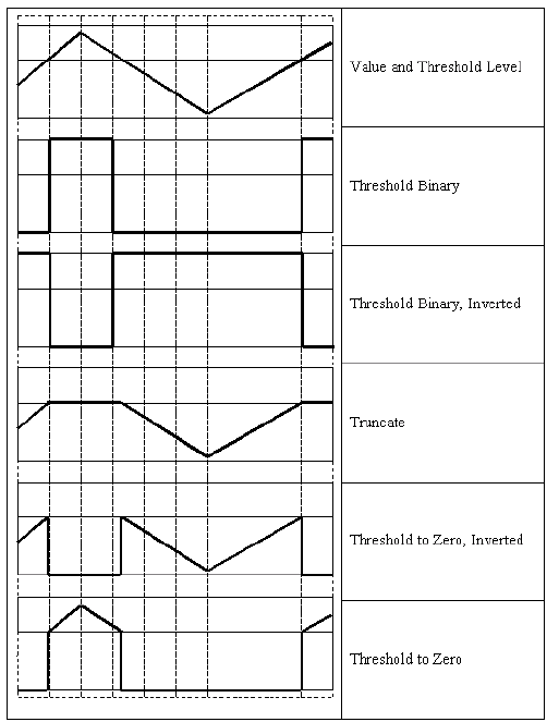
There are several types of thresholding the function supports that are determined by thresholdType:
thresholdType=CV_THRESH_BINARY:
dst(x,y) = maxValue, if src(x,y)>threshold
           0, otherwise

thresholdType=CV_THRESH_BINARY_INV:
dst(x,y) = 0, if src(x,y)>threshold
           maxValue, otherwise

thresholdType=CV_THRESH_TRUNC:
dst(x,y) = threshold, if src(x,y)>threshold
           src(x,y), otherwise

thresholdType=CV_THRESH_TOZERO:
dst(x,y) = src(x,y), if (x,y)>threshold
           0, otherwise

thresholdType=CV_THRESH_TOZERO_INV:
dst(x,y) = 0, if src(x,y)>threshold
           src(x,y), otherwise
And this is the visual description of thresholding types:
Applies adaptive threshold to array
void cvAdaptiveThreshold( const CvArr* src, CvArr* dst, double maxValue,
                          int adaptiveMethod, int thresholdType,
                          int blockSize, double param1 );
CV_THRESH_BINARY and CV_THRESH_BINARY_INV.
CV_ADAPTIVE_THRESH_MEAN_C
or CV_ADAPTIVE_THRESH_GAUSSIAN_C (see the discussion).
CV_THRESH_BINARY,
CV_THRESH_BINARY_INV,
CV_ADAPTIVE_THRESH_MEAN_C and CV_ADAPTIVE_THRESH_GAUSSIAN_C
it is a constant subtracted from mean or weighted mean (see the discussion), though it may be negative.
The function cvAdaptiveThreshold transforms grayscale image to binary image according to the formulae:
thresholdType=CV_THRESH_BINARY:
dst(x,y) = maxValue, if src(x,y)>T(x,y)
           0, otherwise

thresholdType=CV_THRESH_BINARY_INV:
dst(x,y) = 0, if src(x,y)>T(x,y)
           maxValue, otherwise
where TI is a threshold calculated individually for each pixel.
For the method CV_ADAPTIVE_THRESH_MEAN_C it is a mean of blockSize × blockSize
pixel neighborhood, subtracted by param1.
For the method CV_ADAPTIVE_THRESH_GAUSSIAN_C it is a weighted sum (gaussian) of
blockSize × blockSize pixel neighborhood, subtracted by param1.
Performs look-up table transformation on image
CvMat* cvLUT( const CvArr* A, CvArr* B, const CvArr* lut );
The function cvLUT fills the destination array with values of look-up table entries. Indices of the entries are taken from the source array. That is, the function processes each pixel as follows:
B(x,y)=lut[A(x,y)+Δ]where Δ is 0 for 8-bit
unsigned source image type and 128 for 8-bit signed source image type.
Downsamples image
void cvPyrDown( const CvArr* src, CvArr* dst, int filter=CV_GAUSSIAN_5x5 );
CV_GAUSSIAN_5x5 is
currently supported.
The function cvPyrDown performs downsampling step of Gaussian pyramid decomposition. First it convolves source image with the specified filter and then downsamples the image by rejecting even rows and columns.
Upsamples image
void cvPyrUp( const CvArr* src, CvArr* dst, int filter=CV_GAUSSIAN_5x5 );
CV_GAUSSIAN_5x5 is
currently supported.
The function cvPyrUp performs up-sampling step of Gaussian pyramid decomposition. First it upsamples the source image by injecting even zero rows and columns and then convolves result with the specified filter multiplied by 4 for interpolation. So the destination image is four times larger than the source image.
Implements image segmentation by pyramids
void cvPyrSegmentation( IplImage* src, IplImage* dst,
                        CvMemStorage* storage, CvSeq** comp,
                        int level, double threshold1, double threshold2 );
The function cvPyrSegmentation implements image segmentation by pyramids. The
pyramid builds up to the level level. The links between any pixel a on level i
and its candidate father pixel b on the adjacent level are established if
p(c(a),c(b))<threshold1.
After the connected components are defined, they are joined into several
clusters. Any two segments A and B belong to the same cluster, if
p(c(A),c(B))<threshold2. The input
image has only one channel, then
p(c¹,c²)=|c¹-c²|. If the input image has three channels (red,
green and blue), then
p(c¹,c²)=0,3·(c¹r-c²r)+0,59·(c¹g-c²g)+0,11·(c¹b-c²b) .
There may be more than one connected component per a cluster.
src and dst should be 8-bit single-channel or 3-channel images
or equal size
Connected component
    typedef struct CvConnectedComp
    {
        double area; /* area of the segmented component */
        float value; /* gray scale value of the segmented component */
        CvRect rect; /* ROI of the segmented component */
    } CvConnectedComp;
Fills a connected component with given color
void cvFloodFill( CvArr* img, CvPoint seed, double newVal,
                  double lo=0, double up=0, CvConnectedComp* comp=0,
                  int flags=4, CvArr* mask=0 );
#define CV_FLOODFILL_FIXED_RANGE (1 << 16)
#define CV_FLOODFILL_MASK_ONLY   (1 << 17)
CV_RGB macro).
newVal is ignored),
but the fills mask (that must be non-NULL in this case).
img. If not NULL, the function uses and updates the mask, so user takes responsibility of
initializing mask content. Floodfilling can't go across
non-zero pixels in the mask, for example, an edge detector output can be used as a mask
to stop filling at edges. Or it is possible to use the same mask in multiple calls to the function
to make sure the filled area do not overlap.
The function cvFloodFill fills a connected component starting from the seed pixel
where all pixels within the component have close to each other values (prior to filling).
The pixel is considered to belong to the repainted domain if its value I(x,y)
meets the following conditions (the particular cases are specifed after commas):
I(x',y')-lo<=I(x,y)<=I(x',y')+up, grayscale image + floating range
I(seed.x,seed.y)-lo<=I(x,y)<=I(seed.x,seed.y)+up, grayscale image + floating range

I(x',y')r-lor<=I(x,y)r<=I(x',y')r+upr and
I(x',y')g-log<=I(x,y)g<=I(x',y')g+upg and
I(x',y')b-lob<=I(x,y)b<=I(x',y')b+upb, color image + floating range

I(seed.x,seed.y)r-lor<=I(x,y)r<=I(seed.x,seed.y)r+upr and
I(seed.x,seed.y)g-log<=I(x,y)g<=I(seed.x,seed.y)g+upg and
I(seed.x,seed.y)b-lob<=I(x,y)b<=I(seed.x,seed.y)b+upb, color image + fixed range
where
I(x',y') is value of one of pixel neighbors (to be added to the connected
component in case of floating range, a pixel should have at least one neigbor with similar brightness)
Finds contours in binary image
int cvFindContours( CvArr* img, CvMemStorage* storage, CvSeq** firstContour,
                    int headerSize=sizeof(CvContour), CvContourRetrievalMode mode=CV_RETR_LIST,
                    CvChainApproxMethod method=CV_CHAIN_APPROX_SIMPLE );
binary. To get such a binary image
from grayscale, one may use cvThreshold, cvAdaptiveThreshold or cvCanny.
The function modifies the source image content.
method=CV_CHAIN_CODE,
and >=sizeof(CvContour) otherwise.
CV_RETR_EXTERNALretrives only the extreme outer contours
CV_RETR_LISTretrieves all the contours and puts them in the list
CV_RETR_CCOMPretrieves all the contours and organizes them into two-level hierarchy:
top level are external boundaries of the components, second level are bounda
boundaries of the holes
CV_RETR_TREEretrieves all the contours and reconstructs the full hierarchy of
nested contours
CV_CHAIN_CODEoutputs contours in the Freeman chain code. All other methods output polygons
(sequences of vertices).
CV_CHAIN_APPROX_NONEtranslates all the points from the chain code into
points;
CV_CHAIN_APPROX_SIMPLEcompresses horizontal, vertical, and diagonal segments,
that is, the function leaves only their ending points;
CV_CHAIN_APPROX_TC89_L1,CV_LINK_RUNS uses completely different (from the previous methods) algorithm -
linking of horizontal segments of 1's. Only CV_RETR_LIST retrieval mode is allowed by
the method.
The function cvFindContours retrieves contours from the binary image and returns
the number of retrieved contours. The pointer firstContour is filled by the function.
It will contain pointer to the first most outer contour or NULL if no contours is detected (if the image is completely black).
Other contours may be reached from firstContour using h_next and v_next links.
The sample in cvDrawContours discussion shows how to use contours for connected component
detection. Contours can be also used for shape analysis and object recognition - see squares
sample in CVPR 2001 tutorial course located at SourceForge site.
Initializes contour scanning process
CvContourScanner cvStartFindContours( IplImage* img, CvMemStorage* storage,
                                      int headerSize, CvContourRetrievalMode mode,
                                      CvChainApproxMethod method );
method=CV_CHAIN_CODE,
and >=sizeof(CvContour) otherwise.
The function cvStartFindContours initializes and returns pointer to the contour scanner. The scanner is used further in cvFindNextContour to retrieve the rest of contours.
Finds next contour in the image
CvSeq* cvFindNextContour( CvContourScanner scanner );
The function cvFindNextContour locates and retrieves the next contour in the image and returns pointer to it. The function returns NULL, if there is no more contours.
Replaces retrieved contour
void cvSubstituteContour( CvContourScanner scanner, CvSeq* newContour );
The function cvSubstituteContour replaces the retrieved contour, that was returned
from the preceding call of the function cvFindNextContour and stored inside
the contour scanner state, with the user-specified contour. The contour is
inserted into the resulting structure, list, two-level hierarchy, or tree,
depending on the retrieval mode. If the parameter newContour=NULL, the retrieved
contour is not included into the resulting structure, nor all of its children
that might be added to this structure later.
Finishes scanning process
CvSeq* cvEndFindContours( CvContourScanner* scanner );
The function cvEndFindContours finishes the scanning process and returns the pointer to the first contour on the highest level.
Draws contour outlines or interiors in the image
void cvDrawContours( CvArr *image, CvSeq* contour,
                     double external_color, double hole_color,
                     int max_level, int thickness=1,
                     int connectivity=8 );
contour is drawn. If
1, the contour and all contours after it on the same level are drawn. If 2, all
contours after and all contours one level below the contours are drawn, etc.
If the value is negative, the function does not draw the contours following after contour
but draws child contours of contour up to abs(maxLevel)-1 level.
The function cvDrawContours draws contour outlines in the image if thickness>=0
or fills area bounded by the contours if thickness<0.
#include "cv.h"
#include "highgui.h"

int main( int argc, char** argv )
{
    IplImage* src;
    // the first command line parameter must be file name of binary (black-n-white) image
    if( argc == 2 && (src=cvLoadImage(argv[1], 0))!= 0)
    {
        IplImage* dst = cvCreateImage( cvGetSize(src), 8, 3 );
        CvMemStorage* storage = cvCreateMemStorage(0);
        CvSeq* contour = 0;

        cvThreshold( src, src, 1, 255, CV_THRESH_BINARY );
        cvNamedWindow( "Source", 1 );
        cvShowImage( "Source", src );

        cvFindContours( src, storage, &contour, sizeof(CvContour), CV_RETR_CCOMP, CV_CHAIN_APPROX_SIMPLE );
        cvZero( dst );

        for( ; contour != 0; contour = contour->h_next )
        {
            int color = CV_RGB( rand(), rand(), rand() );
            /* replace CV_FILLED with 1 to see the outlines */
            cvDrawContours( dst, contour, color, color, -1, CV_FILLED, 8 );
        }

        cvNamedWindow( "Components", 1 );
        cvShowImage( "Components", dst );
        cvWaitKey(0);
    }
}
Replace CV_FILLED with 1 in the sample below to see the contour outlines
Calculates all moments up to third order of a polygon or rasterized shape
void cvMoments( const CvArr* arr, CvMoments* moments, int isBinary=0 );
The function cvMoments calculates spatial and central moments up to the third order and
writes them to moments. The moments may be used then to calculate gravity center of the shape,
its area, main axises and various shape characeteristics including 7 Hu invariants.
Retrieves spatial moment from moment state structure
double cvGetSpatialMoment( CvMoments* moments, int j, int i );
The function cvGetSpatialMoment retrieves the spatial moment, which in case of image moments is defined as:
Mji=sumx,y(I(x,y)•xj•yi)
where I(x,y) is the intensity of the pixel (x, y).
Retrieves central moment from moment state structure
double cvGetCentralMoment( CvMoments* moments, int j, int i );
The functioncvGetCentralMoment retrieves the central moment, which in case of image moments is defined as:
μij=sumx,y(I(x,y)•(x-xc)j•(y-yc)i),

where xc=M10/M00, yc=M01/M00 - coordinates of the gravity center
Retrieves normalized central moment from moment state structure
double cvGetNormalizedCentralMoment( CvMoments* moments, int x_order, int y_order );
The function cvGetNormalizedCentralMoment retrieves the normalized central moment, which in case of image moments is defined as:
ηij= μij/M00((i+j)/2+1)
Calculates seven Hu invariants
void cvGetHuMoments( CvMoments* moments, CvHuMoments* HuMoments );
The function cvGetHuMoments calculates seven Hu invariants that are defined as:
 h1=η20+η02

 h2=(η20-η02)²+4η11²

 h3=(η30-3η12)²+ (3η21-η03)²

 h4=(η30+η12)²+ (η21+η03)²

 h5=(η30-3η12)(η30+η12)[(η30+η12)²-3(η21+η03)²]+(3η21-η03)(η21+η03)[3(η30+η12)²-(η21+η03)²]

 h6=(η20-η02)[(η30+η12)²- (η21+η03)²]+4η11(η30+η12)(η21+η03)

 h7=(3η21-η03)(η21+η03)[3(η30+η12)²-(η21+η03)²]-(η30-3η12)(η21+η03)[3(η30+η12)²-(η21+η03)²]
These values are proved to be invariants to the image scale, rotation, and reflection except the seventh one, whose sign is changed by reflection.
Finds lines in binary image using Hough transform
CvSeq* cvHoughLines2( CvArr* image, void* lineStorage, int method,
                      double dRho, double dTheta, int threshold,
                      double param1=0, double param2 );
cols/rows contains
a number of lines detected (that is a matrix is truncated to fit exactly the detected lines,
though no data is deallocated - only the header is modified). In the latter case
if the actual number of lines exceeds the matrix size, the maximum possible number of lines is returned
(the lines are not sorted by length, confidence or whatever criteria).
CV_HOUGH_STANDARD - classical or standard Hough transform. Every line is represented by two floating-point numbers
(ρ, θ), where ρ is a distance between (0,0) point and the line, and θ is the angle
between x-axis and the normal to the line. Thus, the matrix must be (the created sequence will
be) of CV_32FC2 type.
CV_HOUGH_PROBABILISTIC - probabilistic Hough transform (more efficient in case if picture contains
a few long linear segments). It returns line segments rather than the whole lines.
Every segment is represented by starting and ending points, and the matrix must be
(the created sequence will be) of CV_32SC4 type.
CV_HOUGH_MULTI_SCALE - multi-scale variant of classical Hough transform.
The lines are encoded the same way as in CV_HOUGH_CLASSICAL.
threshold.
dRho.
(The coarse distance resolution will be dRho and the accurate resolution will be (dRho / param1)).
dTheta.
(The coarse angle resolution will be dTheta and the accurate resolution will be (dTheta / param2)).
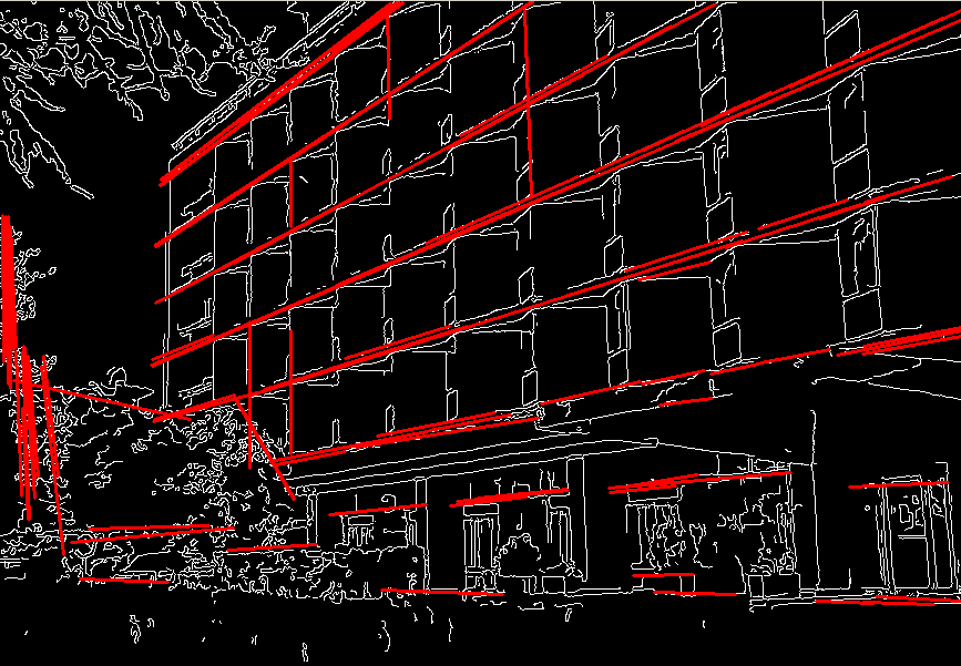
The function cvHoughLines2 implements a few variants of Hough transform for line detection.
/* This is a standalone program. Pass an image name as a first parameter of the program.
   Switch between standard and probabilistic Hough transform by changing "#if 1" to "#if 0" and back */
#include <cv.h>
#include <highgui.h>
#include <math.h>

int main(int argc, char** argv)
{
    IplImage* src;
    if( argc == 2 && (src=cvLoadImage(argv[1], 0))!= 0)
    {
        IplImage* dst = cvCreateImage( cvGetSize(src), 8, 1 );
        IplImage* color_dst = cvCreateImage( cvGetSize(src), 8, 3 );
        CvMemStorage* storage = cvCreateMemStorage(0);
        CvSeq* lines = 0;
        int i;
        cvCanny( src, dst, 50, 200, 3 );
        cvCvtColor( dst, color_dst, CV_GRAY2BGR );
#if 1
        lines = cvHoughLines2( dst, storage, CV_HOUGH_CLASSICAL, 1, CV_PI/180, 150, 0, 0 );

        for( i = 0; i < lines->total; i++ )
        {
            float* line = (float*)cvGetSeqElem(lines,i);
            float rho = line[0];
            float theta = line[1];
            CvPoint pt1, pt2;
            double a = cos(theta), b = sin(theta);
            if( fabs(a) < 0.001 )
            {
                pt1.x = pt2.x = cvRound(rho);
                pt1.y = 0;
                pt2.y = color_dst->height;
            }
            else if( fabs(b) < 0.001 )
            {
                pt1.y = pt2.y = cvRound(rho);
                pt1.x = 0;
                pt2.x = color_dst->width;
            }
            else
            {
                pt1.x = 0;
                pt1.y = cvRound(rho/b);
                pt2.x = cvRound(rho/a);
                pt2.y = 0;
            }
            cvLine( color_dst, pt1, pt2, CV_RGB(255,0,0), 3, 8 );
        }
#else
        lines = cvHoughLines2( dst, storage, CV_HOUGH_PROBABILISTIC, 1, CV_PI/180, 80, 30, 10 );
        for( i = 0; i < lines->total; i++ )
        {
            CvPoint* line = (CvPoint*)cvGetSeqElem(lines,i);
            cvLine( color_dst, line[0], line[1], CV_RGB(255,0,0), 3, 8 );
        }
#endif
        cvNamedWindow( "Source", 1 );
        cvShowImage( "Source", src );

        cvNamedWindow( "Hough", 1 );
        cvShowImage( "Hough", color_dst );

        cvWaitKey(0);
    }
}
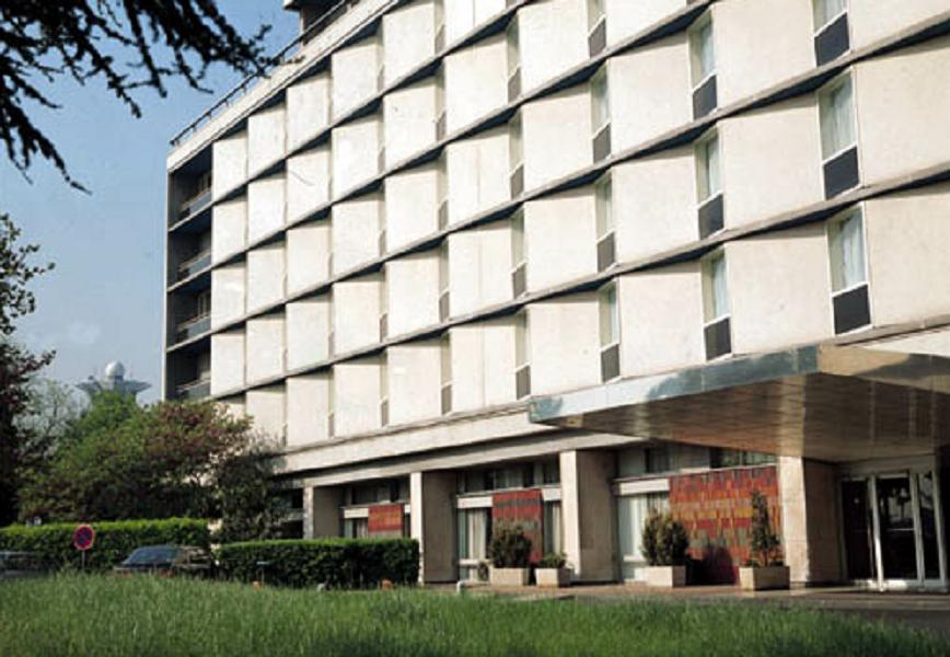
This is the sample picture the function parameters have been tuned for:
And this is the output of the above program in case of probabilistic Hough transform ("#if 0" case):
Calculates distance to closest zero pixel for all non-zero pixels of source image
void cvDistTransform( const CvArr* src, CvArr* dst, CvDisType disType=CV_DIST_L2,
                      int maskSize=3, float* mask=0 );
CV_DIST_L1, CV_DIST_L2, CV_DIST_C or
CV_DIST_USER.
CV_DIST_L1 or
CV_DIST_C the parameter is forced to 3, because 5×5 mask gives the same result
as 3×3 in this case yet it is slower.
The function cvDistTransform calculates the approximated distance from every binary image pixel
to the nearest zero pixel. For zero pixels the function sets the zero distance, for others it finds
the shortest path consisting of basic shifts: horizontal, vertical, diagonal or knight's move (the
latest is available for 5×5 mask). The overal distance is calculated as a sum of these basic distances.
Because the distance function should be symmetric, all the horizontal and vertical shifts must have
the same cost (that is denoted as a), all the diagonal shifts must have the same cost
(denoted b), and all knight's moves' must have the same cost (denoted c).
For CV_DIST_C and CV_DIST_L1 types the distance is calculated precisely,
whereas for CV_DIST_L2 (Euclidian distance) the distance can be calculated only with
some relative error (5×5 mask gives more accurate results), OpenCV uses the values suggested in
[Borgefors86]:
CV_DIST_C (3×3):
a=1, b=1

CV_DIST_L1 (3×3):
a=1, b=2

CV_DIST_L2 (3×3):
a=0.955, b=1.3693

CV_DIST_L2 (5×5):
a=1, b=1.4, c=2.1969
And below are samples of distance field (black (0) pixel is in the middle of white square) in case of user-defined distance:
| 4.5 | 4 | 3.5 | 3 | 3.5 | 4 | 4.5 |
| 4 | 3 | 2.5 | 2 | 2.5 | 3 | 4 |
| 3.5 | 2.5 | 1.5 | 1 | 1.5 | 2.5 | 3.5 |
| 3 | 2 | 1 | 0 | 1 | 2 | 3 |
| 3.5 | 2.5 | 1.5 | 1 | 1.5 | 2.5 | 3.5 |
| 4 | 3 | 2.5 | 2 | 2.5 | 3 | 4 |
| 4.5 | 4 | 3.5 | 3 | 3.5 | 4 | 4.5 |
| 4.5 | 3.5 | 3 | 3 | 3 | 3.5 | 4.5 |
| 3.5 | 3 | 2 | 2 | 2 | 3 | 3.5 |
| 3 | 2 | 1.5 | 1 | 1.5 | 2 | 3 |
| 3 | 2 | 1 | 0 | 1 | 2 | 3 |
| 3 | 2 | 1.5 | 1 | 1.5 | 2 | 3 |
| 3.5 | 3 | 2 | 2 | 2 | 3 | 3.5 |
| 4 | 3.5 | 3 | 3 | 3 | 3.5 | 4 |
Typically, for fast coarse distance estimation CV_DIST_L2, 3×3 mask is used, and for more accurate distance estimation CV_DIST_L2, 5×5 mask is used.
[Borgefors86] Gunilla Borgefors, "Distance Transformations in Digital Images". Computer Vision, Graphics and Image Processing 34, 344-371 (1986).
Muti-dimensional histogram
    typedef struct CvHistogram
    {
        int header_size; /* header's size */
        CvHistType type; /* type of histogram */
        int flags; /* histogram's flags */
        int c_dims; /* histogram's dimension */
        int dims[CV_HIST_MAX_DIM]; /* every dimension size */
        int mdims[CV_HIST_MAX_DIM]; /* coefficients for fast access to element */
        /* &m[a,b,c] = m + a*mdims[0] + b*mdims[1] + c*mdims[2] */
        float* thresh[CV_HIST_MAX_DIM]; /* bin boundaries arrays for every dimension */
        float* array; /* all the histogram data, expanded into the single row */
    struct CvNode* root; /* root of balanced tree storing histogram bins */
        CvSet* set; /* pointer to memory storage (for the balanced tree) */
        int* chdims[CV_HIST_MAX_DIM]; /* cache data for fast calculating */
    } CvHistogram;
Creates histogram
CvHistogram* cvCreateHist( int cDims, int* dims, int type,
                           float** ranges=0, int uniform=1 );
CV_HIST_ARRAY means that histogram data is
represented as an multi-dimensional dense array CvMatND;
CV_HIST_TREE means that histogram data is represented
as a multi-dimensional sparse array CvSparseMat.
uniform parameter value.
The ranges are used for when histogram is calculated or backprojected to determine, which histogram bin
corresponds to which value/tuple of values from the input image[s].
0<=i<cDims ranges[i] is array of two numbers: lower and upper
boundaries for the i-th histogram dimension. The whole range [lower,upper] is split then
into dims[i] equal parts to determine i-th input tuple value ranges for every histogram bin.
And if uniform=0, then i-th element of ranges array contains dims[i]+1 elements:
lower0, upper0, lower1, upper1 == lower2, ..., upperdims[i]-1,
where lowerj and upperj are lower and upper
boundaries of i-th input tuple value for j-th bin, respectively.
In either case, the input values that are beyond the specified range for a histogram bin, are not
counted by cvCalcHist and filled with 0 by cvCalcBackProject.
The function cvCreateHist creates a histogram of the specified size and returns
the pointer to the created histogram. If the array ranges is 0, the histogram
bin ranges must be specified later via the function cvSetHistBinRanges, though
cvCalcHist and cvCalcBackProject may process 8-bit images without setting
bin ranges, they assume equally spaced in 0..255 bins.
Sets bounds of histogram bins
void cvSetHistBinRanges( CvHistogram* hist, float** ranges, int uniform=1 );
The function cvSetHistBinRanges is a stand-alone function for setting bin ranges
in the histogram. For more detailed description of the parameters ranges and
uniform see cvCalcHist function,
that can initialize the ranges as well.
Ranges for histogram bins must be set before the histogram is calculated or
backproject of the histogram is calculated.
Releases histogram
void cvReleaseHist( CvHistogram** hist );
The function cvReleaseHist releases the histogram (header and the data).
The pointer to histogram is cleared by the function. If *hist pointer is already
NULL, the function does nothing.
Clears histogram
void cvClearHist( CvHistogram* hist );
The function cvClearHist sets all histogram bins to 0 in case of dense histogram and removes all histogram bins in case of sparse array.
Makes a histogram out of array
void cvMakeHistHeaderForArray( int cDims, int* dims, CvHistogram* hist,
                               float* data, float** ranges=0, int uniform=1 );
The function cvMakeHistHeaderForArray initializes the histogram, which header and bins are allocated by user. No cvReleaseHist need to be called afterwards. The histogram will be dense, sparse histogram can not be initialized this way.
Queries value of histogram bin
#define cvQueryHistValue_1D( hist, idx0 ) \
    cvGetReal1D( (hist)->bins, (idx0) )
#define cvQueryHistValue_2D( hist, idx0, idx1 ) \
    cvGetReal2D( (hist)->bins, (idx0), (idx1) )
#define cvQueryHistValue_3D( hist, idx0, idx1, idx2 ) \
    cvGetReal3D( (hist)->bins, (idx0), (idx1), (idx2) )
#define cvQueryHistValue_nD( hist, idx ) \
    cvGetRealND( (hist)->bins, (idx) )
The macros cvQueryHistValue_*D return the value of the specified bin of 1D, 2D, 3D or nD histogram. In case of sparse histogram the function returns 0, if the bin is not present in the histogram, and no new bin is created.
Returns pointer to histogram bin
#define cvGetHistValue_1D( hist, idx0 ) \
    ((float*)(cvPtr1D( (hist)->bins, (idx0), 0 ))
#define cvGetHistValue_2D( hist, idx0, idx1 ) \
    ((float*)(cvPtr2D( (hist)->bins, (idx0), (idx1), 0 ))
#define cvGetHistValue_3D( hist, idx0, idx1, idx2 ) \
    ((float*)(cvPtr3D( (hist)->bins, (idx0), (idx1), (idx2), 0 ))
#define cvGetHistValue_nD( hist, idx ) \
    ((float*)(cvPtrND( (hist)->bins, (idx), 0 ))
The macros cvGetHistValue_*D return pointer to the specified bin of 1D, 2D, 3D or nD histogram. In case of sparse histogram the function creates a new bins and fills it with 0, if it does not exists.
Finds minimum and maximum histogram bins
void cvGetMinMaxHistValue( const CvHistogram* hist,
                           float* minVal, float* maxVal,
                           int* minIdx =0, int* maxIdx =0);
hist->c_dims elements to store the coordinates.
hist->c_dims elements to store the coordinates.
The function cvGetMinMaxHistValue finds the minimum and maximum histogram bins and their positions. In case of several maximums or minimums the earliest in lexicographical order extrema locations are returned.
Normalizes histogram
void cvNormalizeHist( CvHistogram* hist, double factor );
The function cvNormalizeHist normalizes the histogram bins by scaling them,
such that the sum of the bins becomes equal to factor.
Thresholds histogram
void cvThreshHist( CvHistogram* hist, double thresh );
The function cvThreshHist clears histogram bins that are below the specified level.
Compares two dense histograms
double cvCompareHist( const CvHistogram* H1, const CvHistogram* H2,
                      CvCompareMethod method );
The function cvCompareHist compares two histograms using specified method and returns the comparison result. It processes as following:
Correlation (method=CV_COMP_CORREL):
d(H1,H2)=sumI(H'1(I)•H'2(I))/sqrt(sumI[H'1(I)2]•sumI[H'2(I)2])
where
H'k(I)=Hk(I)-1/N•sumJHk(J) (N=number of histogram bins)

Chi-Square (method=CV_COMP_CHISQR):
d(H1,H2)=sumI[(H1(I)-H2(I))/(H1(I)+H2(I))]

Intersection (method=CV_COMP_INTERSECT):
d(H1,H2)=sumImax(H1(I),H2(I))
Note, that the function can operate on dense histogram only. To compare sparse histogram or more general sparse configurations of weighted points, consider cvCalcEMD function.
Copies histogram
void cvCopyHist( CvHistogram* src, CvHistogram** dst );
The function cvCopyHist makes a copy of the histogram. If the second histogram
pointer *dst is NULL, a new histogram of the same size as src is created.
Otherwise, both histograms must have equal types and sizes.
Then the function copies the source histogram bins values to destination histogram and
sets the same as src's value ranges.
Calculates histogram of image(s)
void cvCalcHist( IplImage** img, CvHistogram* hist,
                 int doNotClear=0, const CvArr* mask=0 );
The function cvCalcHist calculates the histogram of one or more single-channel images. The elements of a tuple that is used to increment a histogram bin are taken at the same location from the corresponding input images.
#include <cv.h>
#include <highgui.h>

int main( int argc, char** argv )
{
    IplImage* src;
    if( argc == 2 && (src=cvLoadImage(argv[1], 1))!= 0)
    {
        IplImage* h_plane = cvCreateImage( cvGetSize(src), 8, 1 );
        IplImage* s_plane = cvCreateImage( cvGetSize(src), 8, 1 );
        IplImage* v_plane = cvCreateImage( cvGetSize(src), 8, 1 );
        IplImage* planes[] = { h_plane, s_plane };
        IplImage* hsv = cvCreateImage( cvGetSize(src), 8, 3 );
        int h_bins = 30, s_bins = 32;
        int hist_size[] = {h_bins, s_bins};
        float h_ranges[] = { 0, 180 }; /* hue varies from 0 (~0°red) to 180 (~360°red again) */
        float s_ranges[] = { 0, 255 }; /* saturation varies from 0 (black-gray-white) to 255 (pure spectrum color) */
        float* ranges[] = { h_ranges, s_ranges };
        int scale = 10;
        IplImage* hist_img = cvCreateImage( cvSize(h_bins*scale,s_bins*scale), 8, 3 );
        CvHistogram* hist;
        float max_value = 0;
        int h, s;

        cvCvtColor( src, hsv, CV_BGR2HSV );
        cvCvtPixToPlane( hsv, h_plane, s_plane, v_plane, 0 );
        hist = cvCreateHist( 2, hist_size, CV_HIST_ARRAY, ranges, 1 );
        cvCalcHist( planes, hist, 0, 0 );
        cvGetMinMaxHistValue( hist, 0, &max_value, 0, 0 );
        cvZero( hist_img );

        for( h = 0; h < h_bins; h++ )
        {
            for( s = 0; s < s_bins; s++ )
            {
                float bin_val = cvQueryHistValue_2D( hist, h, s );
                int intensity = cvRound(bin_val*255/max_value);
                cvRectangle( hist_img, cvPoint( h*scale, s*scale ),
                             cvPoint( (h+1)*scale - 1, (s+1)*scale - 1),
                             CV_RGB(intensity,intensity,intensity), /* graw a grayscale histogram.
                                                                       if you have idea how to do it
                                                                       nicer let us know */
                             CV_FILLED );
            }
        }

        cvNamedWindow( "Source", 1 );
        cvShowImage( "Source", src );

        cvNamedWindow( "H-S Histogram", 1 );
        cvShowImage( "H-S Histogram", hist_img );

        cvWaitKey(0);
    }
}
Calculates back projection
void cvCalcBackProject( IplImage** img, CvArr* backProject, const CvHistogram* hist );
The function cvCalcBackProject calculates the back project of the histogram. For each tuple of pixels at the same position of all input single-channel images the function puts the value of the histogram bin, corresponding to the tuple, to the destination image. In terms of statistics, the value of each output image pixel is probability of the observed tuple given the distribution (histogram). For example, to find a red object in the picture, one may do the following:
Locates a template within image by histogram comparison
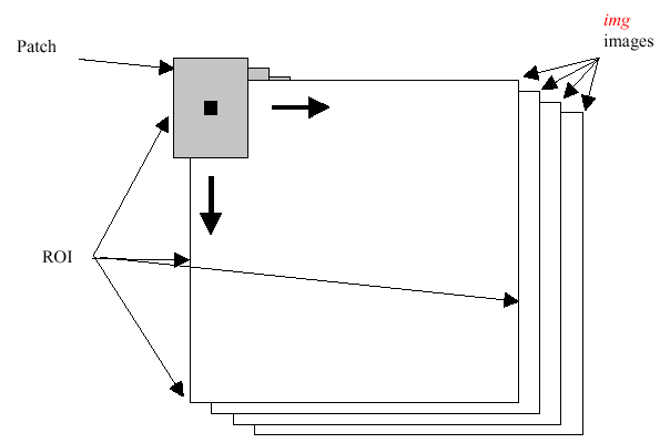
void cvCalcBackProjectPatch( IplImage** img, CvArr* dst,
                             CvSize patchSize, CvHistogram* hist,
                             int method, float normFactor );
The function cvCalcBackProjectPatch calculates back projection by comparing
histograms of the source image patches with the given histogram. Taking
measurement results from some image at each location over ROI creates an array
img. These results might be one or more of hue, x derivative, y derivative,
Laplacian filter, oriented Gabor filter, etc. Each measurement output is
collected into its own separate image. The img image array is a collection of
these measurement images. A multi-dimensional histogram hist is constructed by
sampling from the img image array. The final histogram is normalized. The hist
histogram has as many dimensions as the number of elements in img array.
Each new image is measured and then converted into an img image array over a
chosen ROI. Histograms are taken from this img image in an area covered by a
"patch" with anchor at center as shown in the picture below.
The histogram is normalized using the parameter norm_factor so that it
may be compared with hist. The calculated histogram is compared to the model
histogram; hist uses the function cvCompareHist with the comparison method=method).
The resulting output is placed at the location corresponding to the patch anchor in
the probability image dst. This process is repeated as the patch is slid over
the ROI. Iterative histogram update by subtracting trailing pixels covered by the patch and adding newly
covered pixels to the histogram can save a lot of operations, though it is not implemented yet.
Divides one histogram by another
void  cvCalcProbDensity( const CvHistogram* hist1, const CvHistogram* hist2,
                         CvHistogram* histDens, double scale=255 );
The function cvCalcProbDensity calculates the object probability density from the two histograms as:
histDens(I)=0  if hist1(I)==0
            scale  if hist1(I)!=0 && hist2(I)>hist1(I)
            hist2(I)*scale/hist1(I) if hist1(I)!=0 && hist2(I)<=hist1(I)
So the destination histogram bins are within [0,scale).
Computes "minimal work" distance between two weighted point configurations
float cvCalcEMD2( const CvArr* signature1, const CvArr* signature2, CvDisType distType,
                  float (*distFunc)(const float* f1, const float* f2, void* userParam ),
                  const CvArr* costMatrix, CvArr* flow,
                  float* lowerBound, void* userParam );
size1×dims+1 floating-point matrix.
Each row stores the point weight followed by the point coordinates. The matrix is allowed to
have a single column (weights only) if the user-defined cost matrix is used.
signature1, though the number
of rows may be different. The total weights may be different, in this case an extra "dummy" point
is added to either signature1 or signature2.
CV_DIST_L1, CV_DIST_L2, and CV_DIST_C stand for one of
the standard metrics; CV_DIST_USER means that a user-defined function distFunc or
pre-calculated costMatrix is used.
size1×size2 cost matrix.
At least one of costMatrix and distFunc must be NULL.
Also, if a cost matrix is used, lower boundary (see below) can not be calculated,
because it needs a metric function.
size1×size2 flow matrix: flowij is a flow
from i-th point of signature1 to j-th point of signature2
The function cvCalcEMD2 computes earth mover distance and/or a lower boundary of the distance between the two weighted point configurations. One of the application desctibed in [RubnerSept98] is multi-dimensional histogram comparison for image retrieval. EMD is a transportation problem that is solved using some modification of simplex algorithm, thus the complexity is exponential in the worst case, though, it is much faster in average. In case of real metric the lower boundary can be calculated even faster (using linear-time algorithm) and it can be used to determine roughly whether the two signatures are far enough so that they cannot relate to the same object.
[RubnerSept98] Y. Rubner. C. Tomasi, L.J. Guibas. The Earth Mover's Distance as a Metric for Image Retrieval. Technical Report STAN-CS-TN-98-86, Department of Computer Science, Stanford University, September 1998.
Compares template against overlapped image regions
void cvMatchTemplate( const CvArr* I, const CvArr* T,
                      CvArr* result, int method );
I is
W×H and T is w×h then R must
be W-w+1×H-h+1.
The function cvMatchTemplate is similiar to cvCalcBackProjectPatch.
It slids through I, compares w×h
patches against T using the specified method and stores the comparison results
to result. Here are the formular for the different comparison methods one may use
(the summation is done over template and/or the image patch: x'=0..w-1, y'=0..h-1):
method=CV_TM_SQDIFF:
R(x,y)=sumx',y'[T(x',y')-I(x+x',y+y')]2

method=CV_TM_SQDIFF_NORMED:
R(x,y)=sumx',y'[T(x',y')-I(x+x',y+y')]2/sqrt[sumx',y'T(x',y')2•sumx',y'I(x+x',y+y')2]

method=CV_TM_CCORR:
R(x,y)=sumx',y'[T(x',y')•I(x+x',y+y')]

method=CV_TM_CCORR_NORMED:
R(x,y)=sumx',y'[T(x',y')•I(x+x',y+y')]/sqrt[sumx',y'T(x',y')2•sumx',y'I(x+x',y+y')2]

method=CV_TM_CCOEFF:
R(x,y)=sumx',y'[T'(x',y')•I'(x+x',y+y')],

where T'(x',y')=T(x',y') - 1/(w•h)•sumx",y"T(x",y") (mean template brightness=>0)
      I'(x+x',y+y')=I(x+x',y+y') - 1/(w•h)•sumx",y"I(x+x",y+y") (mean patch brightness=>0)

method=CV_TM_CCOEFF_NORMED:
R(x,y)=sumx',y'[T'(x',y')•I'(x+x',y+y')]/sqrt[sumx',y'T'(x',y')2•sumx',y'I'(x+x',y+y')2]
After the function finishes comparison, the best matches can be found as global minimums (CV_TM_SQDIFF*)
or maximums (CV_TM_CCORR* and CV_TM_CCOEFF*) using cvMinMaxLoc function.