Difference Equations and Impulse Responses

Contents

1. Sample waveform at 32 kHz

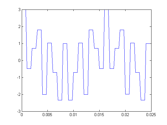
t = [0:1/32000:1];
xc = 2*cos(6000*pi*t) + cos(1000*pi*t);
plot(t(1:100),xc(1:100))

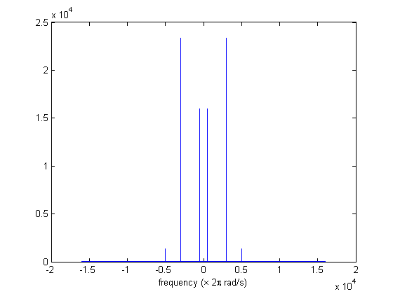
plot([-16000:15999],fftshift(abs(fft(xc(1:4*8000)))))
xlabel('frequency (\times 2\pi rad/s)')

% There is one frequency component at 3 kHz and one at 500 Hz according to
% the function and the graph.  The 3 kHz component is twice as high as the
% 500 Hz one in the function and the graph.

2. Sample at 8 kHz

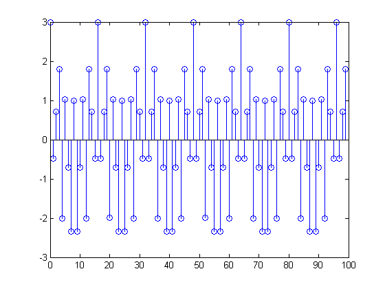
T = 1/8000;
n = [0:8000];
x = 2*cos(6000*pi*n*T) + cos(1000*pi*n*T);

stem([0:99],x(1:100))

plot([-4000:3999]/8000,fftshift(abs(fft(x(1:8000)))))
xlabel('frequency (\times 2\pi rad/sample)')

% Aliasing does not occur, since the sampling rate is more than twice the
% highest frequency.  The graph is just a frequency-axis-scaled version of
% the previous one with scaled height.

3. Sample at 4 kHz

t = [0:1/4000:1];
x4k = 2*cos(6000*pi*t) + cos(1000*pi*t);
plot([-2000:1999]/4000,fftshift(abs(fft(x4k(1:4000)))))

% This signal is aliased, since the sampling frequency 4 kHz is not twice
% as high as the highest frequency 3 kHz.  The 3 kHz signal wraps around to
% -4 + 3 = -1 kHz and 4-3=1 kHz.  The 500 Hz component is not aliased.
% The aliased components show up as +- 1000/4000 = +- 0.25 (*2pi) rad/sample.

4. Reconstruct #1 with ZOH

xzoh = x(1+floor([0:4*length(x)-1]/4));
plot(t(1:100),xzoh(1:100))

plot([-16000:15999],fftshift(abs(fft(xzoh(1:4*8000)))))
xlabel('frequency (\times 2\pi rad/s)')

% The higher frequencies due to replicating the baseband spectrum are
% apparent.  Since the waveform is extended with a pulse, the higher-
% frequency copies are attenuated.

h = fir1(31,1/4);
xr = filter(h,1,xzoh);
plot(t(1:100),xzoh(1:100),t(1:100),xr(18:117),t(1:100),xc(1:100))

plot([-16000:15999],fftshift(abs(fft(xr(1:4*8000)))))
xlabel('frequency (\times 2\pi rad/s)')

% Most of the spectral copies are filtered out, although not perfectly.

5. Play the sounds

soundsc(xc,32000)
soundsc(xr,32000)
soundsc(xzoh,32000)

% The ZOH signal sounds different due to the higher frequencies.  The
% others are quite similar.

wavwrite(xc/max(abs(xc)),32000,'xc.wav')
wavwrite(xr/max(abs(xr)),32000,'xr.wav')
wavwrite(xzoh/max(abs(xzoh)),32000,'xzoh.wav')

Warning: Data clipped during write to file:xc.wav
Warning: Data clipped during write to file:xr.wav
Warning: Data clipped during write to file:xzoh.wav

Published with MATLAB® 7.0.1