
This project will help you to become more familiar with difference equations by exploring their characteristics in both the time and frequency domains.
Let
This difference equation can be implemented using the filter command. Find the vectors a and b that represent the difference equation above for the filter command.
a = [1 -0.5];
b = [0.1 0.8 0.8];
Calculate h[n] analytically for the difference equation above. Hint: You may find the residuez function useful.

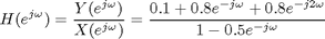

impulse = [1 zeros(1,99)];
h = filter(b,a,impulse);
stem([0:length(h)-1],h)
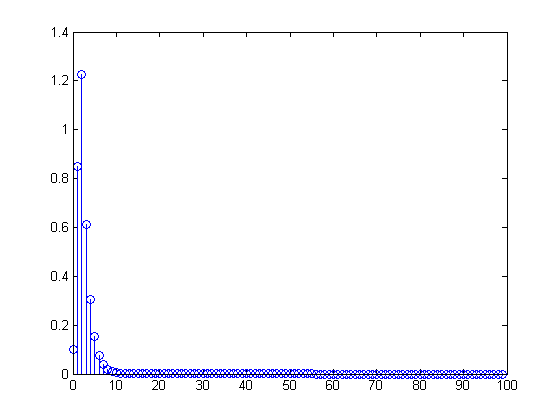
pulse = [ones(1,9) zeros(1,91)];
pulse_filt = filter(b,a,pulse);
pulse_conv = conv(h,pulse);

stem([0:length(pulse_filt)-1],pulse_filt)
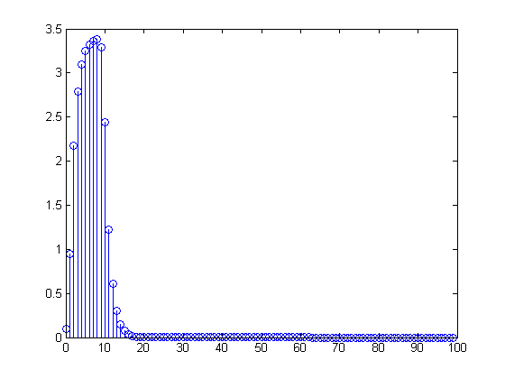
stem([0:length(pulse_conv)-1],pulse_conv)
Visible difference is only in length. However, there are very tiny differences due to truncating the IIR response with filter
stem([0:length(pulse_filt)-1],pulse_filt-pulse_conv(1:length(pulse_filt)))
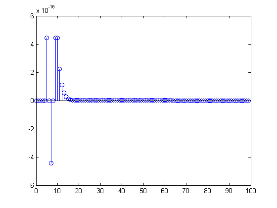
% See #2.
freqz(b,a)
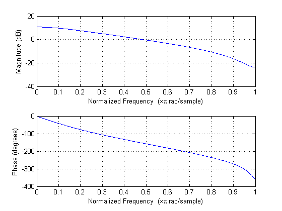
The system is lowpass.
x1 = cos(0.1*pi*[0:99]);
x2 = cos(0.8*pi*[0:99]);

x1filt = filter(b,a,x1);
x2filt = filter(b,a,x2);

stem([0:length(x1filt)-1],x1filt)
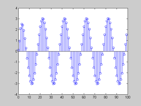
stem([0:length(x2filt)-1],x2filt)
x1 is amplified, but x2 is attenuated
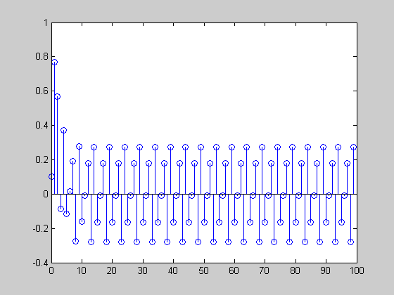
% generate sequence

n = [0:100];
z = 0.5.^n;
zn = n.*z; % time-domain effect
Zf = fft(z); % sampled DTFT of z, where $$\omega = \frac{2\pi}{101}$$
Znf = fft(zn); % sampled DTFT of zn
Zfdiff = j*diff([Zf(end) Zf]); % approximating derivative by difference
Zfdiff = Zfdiff*101/(2*pi); % scaling due to omega vs. k
subplot(2,1,1)
plot(abs(Znf))
subplot(2,1,2)
plot(abs(Zfdiff))
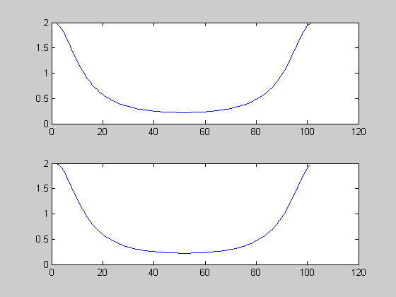
These are approximately the same, as the theory tells us