Using Streamtraces for Current Flow Visualization in Sentaurus – A SiGe HBT Example
First google “streamtraces tecplot” so you have a good idea of the definition – we discussed this today in class – essentially the path of a massless particle when put in a “vector” field – for us, that typically means “current density” “field”.
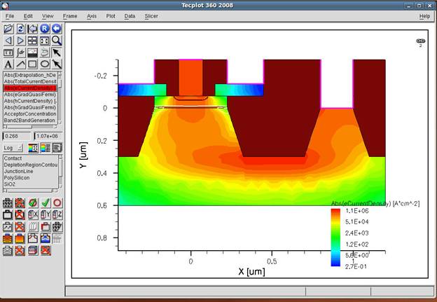
First load in your solution file, select eCurrentDensity – make sure you select “/vector” in the plot section of your _des.cmd file – see our example input files. The color indicates magnitude of current density at each location, the next question is what about the direction – you can use arrow, but the picture gets quite messy when all the arrows overlap with each other – tecplot does this. It does not provide information on the overall current flow path (lines) either. Streamtrace comes into play here.
To show streamtrace(s), go to Plot -> Streamtraces , and specify a point of observation, then the program will trace out the “streamtrace” passing through that point, as shown below:
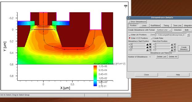
In the above picture, we specified x=0, y=0, and chose to “trace” it in both directions. We end up with a “line” showing the trace of eCurrent from emitter contact to collector contact – the electron transport between E and C in a bipolar transistor, in 2-D, in a very clear way.
You can select “Create Rake” to get multiple lines – experiment with choice of start and end position of the Rake:
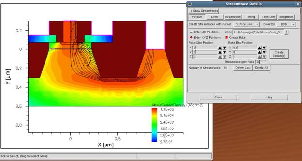
Always remember the magnitude is indicated by the contour / color!
A very nice way to precisely show the physics behind emitter current crowding effect and distributive nature of base resistance calculations is to examine the hole current density streamtraces:
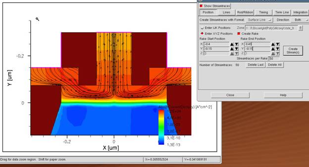
The 2D nature of hole current flow is crystal clear in this picture.
Holes must first flow laterally (under the emitter), and then flow vertically into the emitter. NOT all the base current flows through the whole emitter width, which is why there is the 1/3 or 1/12 factor in our base resistance calculation (intrinsic base resistance).