Note: This page is primarily written as a way of sharing data with project collaborators, and is therefore not entirely self-explanatory. However, if your are interested in more information, please contact:
Dr. Thaddeus Roppel (Auburn University) troppel@eng.auburn.edu or
Dr. Denise Wilson (University of Washington) wilson@ee.washington.edu
Also, visit the Sensor Fusion Lab at Auburn University.
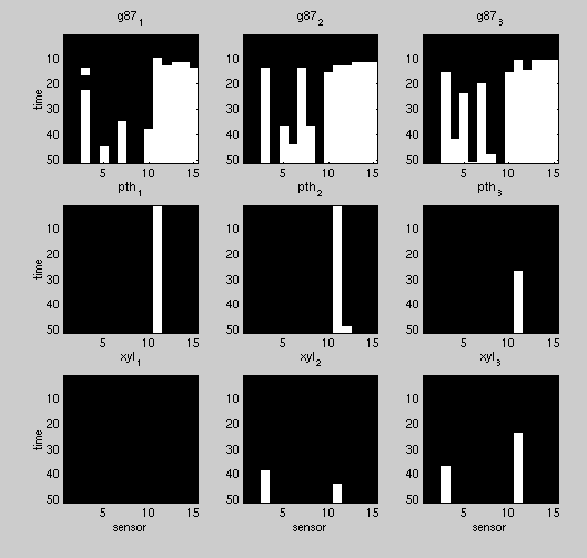
The figure below shows the neuromorphic representation of the response of 15 tin-oxide sensors to nine odor presentations. There are three presentations each of three samples:
In each subplot, the horizontal axis is the sensor number (1-15).
The vertical axis is time, running from t=0 at the top to t=51 sample intervals at the bottom. The sensor output voltages (raw data) were sampled approximately every 0.5 seconds
The raw data (0 to 5V) were thresholded at 2V, so a white pixel indicates that a given sensor output exceeds 2V. Generally, the sensor responses are monotonically increasing with time so it is rare for a sensor to drop back below threshold once it has crossed.
An Elman recurrent back-propagation network was trained on the second presentation of each odor (g87_2, pth_2, xyl_2). The network was designed with 15 hidden layer nodes and three output nodes, one for each possible output (G for gasoline, P for paint thinner, and X for xylene). The network was trained for 1500 iterations (approx. 15 minutes on my abacus alias Sparc-whatever).
The figure below shows the result of presenting the training data back to the trained network. This should not be much of a challenge for the net, and indeed the response is essentially perfect. In this plot and those to follow, you can draw an imaginary horizontal line at an output value of 0.5 to get a binary decision threshold. The horizontal axis is time measured in units of PATTERN LENGTH, where one pattern length is 51 samples (i.e., the length of time one odor is presented to the net). For example, the input sequence (g2 p2 x2) is 3 pattern lengths long, and is a shorthand way of indicating that the odors are presented in the order g87_2, pth_2, xyl_2. Each subplot shows the output of the indicated output neuron. Thus if the net detects gasoline, output G will be HIGH (greater than 0.5), and outputs P and X will be LOW (less than 0.5).
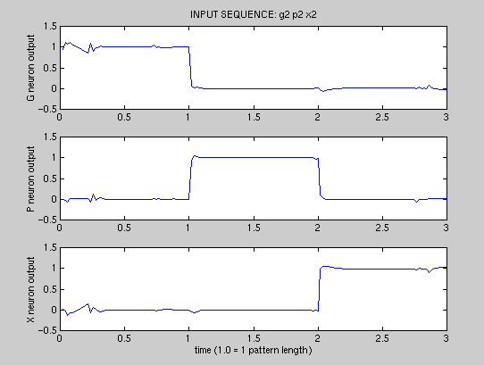
It can be seen that only output G fires during the first pattern length period, when gasoline (g87_2) is being presented. Then only output P fires during the second pattern length period when paint thinner (pth_2) is being presented. Finally, output X fires exclusively when xylene is presented (xyl_2).
For more of a challenge, we now present the same samples in reverse order. Since this neural net is time-dependent, the results might be quite interesting.
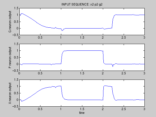
In fact we see that the net takes a significant amount of time during the first pattern length interval to correctly recognize xylene, but it eventually does so. During the second pattern length interval, P is properly recognized. During the third interval, gasoline is recognized, although here again there is a non-negligible recognition time.
Now for even more of a challenge, let's present the net with samples it has never seen before. We will use the input sequence (g1 p1 x1). These are samples of the same substances the net was trained on, but different presentations. By looking back at the 3x3 grid of image maps at the top of this page, you can see that these (shown in the first column) are similar, but certainly not identical to the training samples (g2, p2, x2) in the second column.
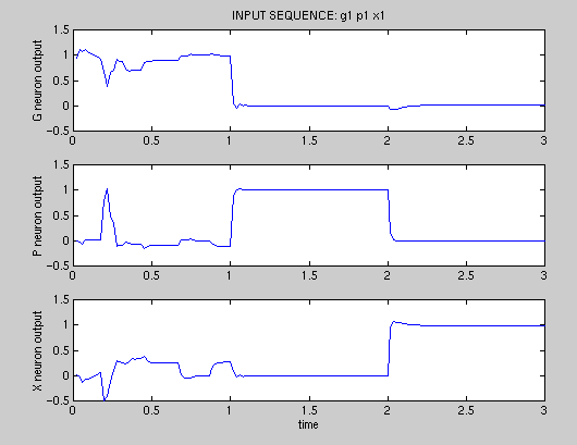
Remarkably, our brave little net does a superb job of recognizing these new samples, except for a little confusion during the first pattern interval.
Finally, just so it doesn't seem too good to be true, we will show an example where the net falls off the mark a bit. Next we present the other samples the net has not yet seen, (g3 p3 x3) shown in column 3 of the 3x3 image map grid at the top of this page. Again, these are similar but not identical to the training data.
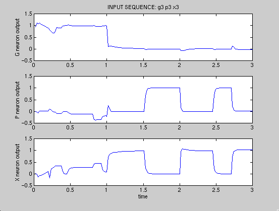
Notice that the G neuron responds correctly to gasoline at all times. But the P and X neurons indicate confusion during the 2nd and 3rd pattern intervals. Note, however, that P and X are mutually exclusive- they are never both high or both low. The reason for this confusion is fairly clear upon close examination of the input data patterns, keeping in mind that the input data is being presented to the network serially,so the net can't know what it has not seen yet. One way to get a feel for this is to slide a piece of paper downward across the input data images and try to decide which sample you are viewing just based on what you can see at any given time.